Mathematics – Page 2 – LeftAsExercise

Grover’s algorithm – unstructured search with a quantum computer

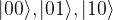
In the last post, we have looked at the Deutsch-Jozsa algorithm that is considered to be the first example of a quantum algorithm that is structurally more efficient than any classical algorithm can probably be. However, the problem solved by the algorithm is rather special. This does, of course, raise the question whether a similar speed-up can be achieved for problems that are more relevant to practical applications.

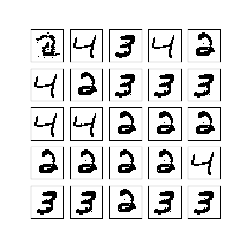
In this post, we will discuss an algorithm of this type – Grover’s algorithm. Even though the speed-up provided by this algorithm is rather limited (which is of a certain theoretical interest in its own right), the algorithm is interesting due to its very general nature. Roughly speaking, the algorithm is concerned with an unstructured search. We are given a set of N = 2ⁿ elements, labeled by the numbers 0 to 2^n-1, exactly one of which having a property denoted by P. We can model this property as a binary valued function P on the set $\{0,N-1\}$ that is zero on all but one elements. The task is to locate the element x₀ for which P(x₀) is true.

Grover’s algorithm

Grover’s algorithm presented in [1] proceeds as follows to locate this element. First, we again apply the Hadamard-Walsh operator W to the state $|0 \rangle$ of an n-qubit system to obtain a superposition of all basis states. Then, we iteratively apply the following sequence of operations.

Apply a conditional phase shift S, i.e. apply the unique unitary transformation that maps $|x \rangle$ to $(-1)^{f(x)} |x \rangle$ .
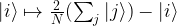
Apply the unitary transformation D called diffusion that we will describe below

Finally, after a defined number of outcomes, we perform a measurement which will collaps the system into one of the states $|x \rangle$ . We claim – and will see why this is true below – that for the right number of iterations, this value x will, with a high likelihood, be the solution to our problem, i.e. equal to x₀.

Before we can proceed, we need to define the matrix D. This matrix is $\frac{2}{N} - 1$ along the diagonal, with N = 2ⁿ, and $\frac{2}{N}$ away from the diagonal. In terms of basis vectors, the mapping is given by

$|i \rangle \mapsto \frac{2}{N} (\sum_j |j \rangle) - |i \rangle$

Consequently, we see that

$D \sum_i a_i |i \rangle = \sum_i (2 \bar{a} - a_i) |i \rangle$

where $\bar{a}$ is the average across the amplitudes $a_i$ . Thus geometrically, the operation D performs an inversion around the average. Grover shows that this operation can be written as minus a Hadamard-Walsh operation followed by the operation that flips the sign for $|0 \rangle$ , followed by a second Hadamard-Walsh transformation.

For the sake of completeness, let us also briefly discuss the first transformation employed by the algorithm, the conditional phase shift. We have already seen a similar transformation while studying the Deutsch-Jozsa algorithm. In fact, we have shown in the respective blog post that the circuit displayed below (with the notation slightly changed)

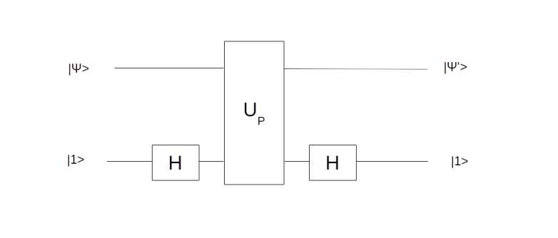
performs the required operation

$|\psi \rangle = \sum_x a_x |x \rangle \mapsto |\psi' \rangle = \sum_x a_x (-1)^{P(x)} |x \rangle$

Let us now see how why Grover’s algorithm works. Instead of going through the careful analysis in [1], we will use bar charts to visualize the quantum states (exploiting that all involved matrices are actually real valued).

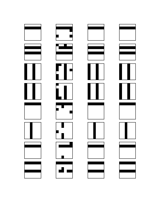
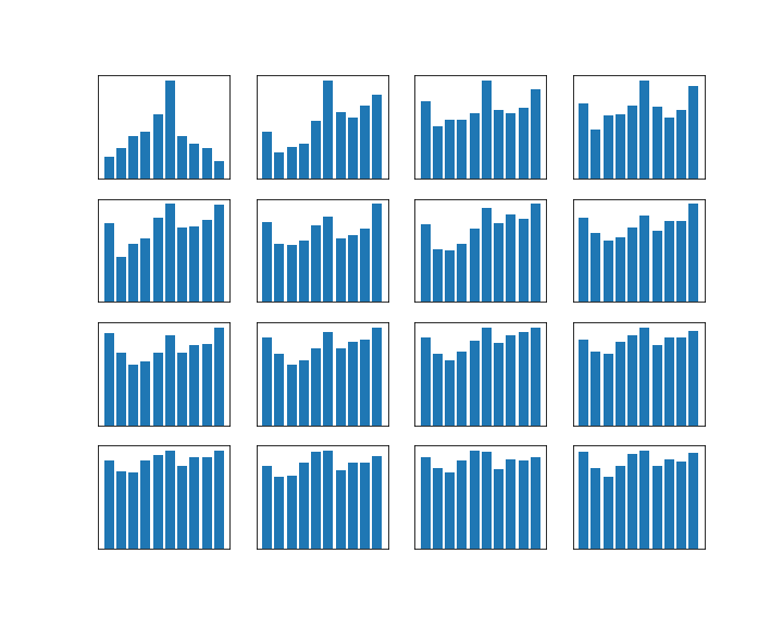
It is not difficult to simulate the transformation in a simple Python notebook, at least for small values of N. This script performs several iterations of the algorithm and prints the result. The diagrams below show the outcome of this test.

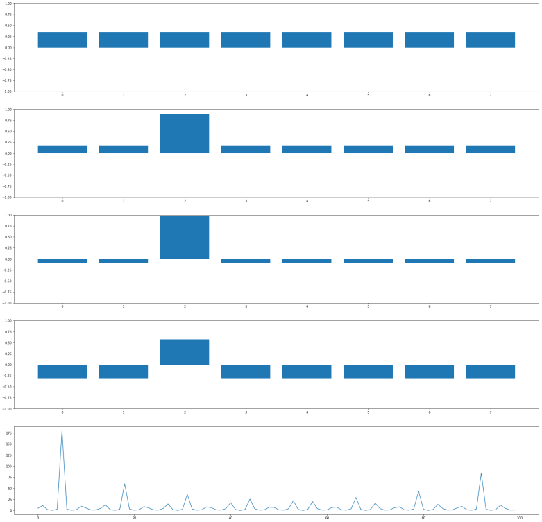
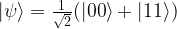
Let us go through the diagrams one by one. The first diagram shows the initial state of the algorithm. I have used 3 qubits, i.e. n = 3 and N = 8. The initial state, after applying the Hadamard-Walsh transform to the zero state, is displayed in the first line. As expected, all amplitudes are equal to 1 over the square root of eight, which is approximately 0.35, i.e. we have a balanced superposition of all states.

We now apply one iteration of the algorithm. First, we apply the conditional phase flip. The element we are looking for is in this case located at x = 2. Thus, the phase flip will leave all basis vectors unchanged except for $|2 \rangle$ and it will change the amplitude of this vector to – 0.35. This will change the average amplitude to a value slightly below 0.35. If we now perform the inversion around the average, the amplitudes of all basis vectors different from $|2 \rangle$ will actually decrease, whereas the amplitude of $|2 \rangle$ will increase. The result is displayed in the second line of the diagram.

Thus, what really happens in this case is an amplitude amplification – we increase the amplitude of one component of the superposition while decreasing all the others.

The next few lines show the result of repeating these two steps. We see that after the second iteration, almost all of the amplitude is concentrated on the vector $|2 \rangle$ , which represents the solution we are looking for. If we now perform a measurement, the result will be 2 with a very high probability!

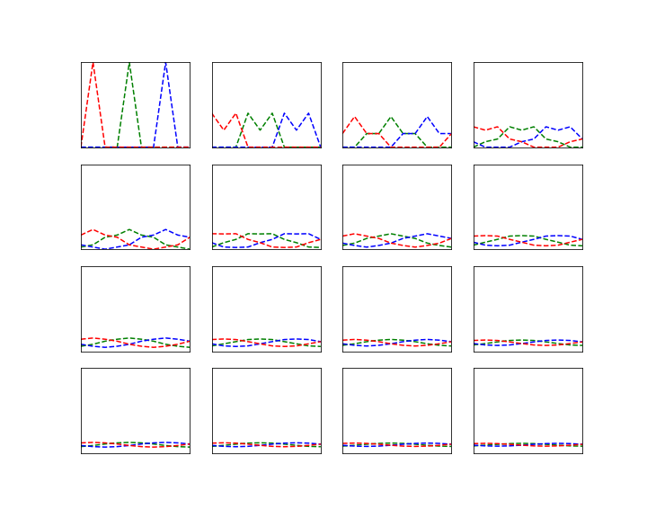
It is interesting to see that when we perform one more iteration, the difference between the amplitude of the solution and the amplitudes of all other components decreases again. Thus the correct choice for the number of iterations is critical to make the algorithm work. In the last line, we have plotted the difference between the amplitude of $|2 \rangle$ and the other amplitudes (more precisely, the ratio between the amplitude of $|2 \rangle$ and the second largest amplitude) on the y-axis for the different number of iterations on the x-axis. We see that the optimal number of iterations is significantly below 10 (actually five iterations give the best result in this case), and more iterations decrease the likelihood of getting the correct result out of the measurement again. In fact, a careful analysis carried out in [2] shows that for large values of N, the best number of iterations is given by $\frac{\pi}{4} \sqrt{N}$ , and that doubling the number of iterations does in general lead to a less optimal result.

Generalizations and amplitude amplification

In a later paper ([3]), Grover describes a more general setup which is helpful to understand the basic reason why the algorithm works – the amplitude amplification. In this paper, Grover argues that given any unitary transformation U and a target state (in our case, the state representing the solution to the search problem), the probability to meet the target state by applying U to a given initial state can be amplified by a sequence of operations very much to the one considered above. We will not go into details, but present a graphical representation of the algorithm.

So suppose that we are given an n-qubit quantum system and two basis vectors – the vector t representing the target state and an initial state s. In addition, assume we are given a unitary transformation U. The goal is to reach t from s by subsequently applying U itself and a small number of additional gates.

Grover considers the two-dimensional subspace spanned by the vectors s and U^-1t. If, within this subspace, we ever manage to reach U^-1t, then of course one more application of U will move us into the desired target state.

Now let us consider the transformation

$Q = - I_s U^{-1} I_t U$

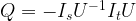
where I_x denotes a conditional phase shift that flips the phase on the vector $|x \rangle$ . Grover shows that this transformation does in fact leave our two-dimensional subspace invariant, as indicated in the diagram below.

He then proceeds to show that for sufficiently small values of the matrix element U_ts, the action of Q on this subspace can approximately be described as a rotation by the angle $\frac{2}{|U_{ts}|}$ . Applying the operation Q n times will then approximately result in a superposition of the form

$\cos (\frac{2n}{|U_{ts}|})|s \rangle + a U^{-1}|t \rangle$

Thus if we can make the first coefficient very small, i.e. if $\frac{4n}{|U_{ts}|}$ is close to a multiple of $\pi$ , then one application of U will take our state to a state very close to t.

Let us link this description to the version of the Grover algorithm discussed above. In this version, the initial state s is the state $|0 \rangle$ . The transformation U is the Hadamard-Walsh transformation W. The target state is $|x_0 \rangle$ where x₀ is the solution to the search problem. Thus the operation I_t is the conditional phase shift that we have denoted by S earlier. In addition, Grover shows in [1] already that the diffusion operator D can be expressed as -W I₀ W. Now suppose we apply the transformation Q n times to the initial state and then apply U = W once more. Then our state will be

$W Q \dots Q |0 \rangle$

This can be written as

$W (-I_0 W S W) (-I_0 W S W) \dots (-I_0 W S W) |0 \rangle$

Regrouping this and using the relation D = -W I₀ W, we see that this is the same as

$- (W I_0 W) S (- W I_0 W) S \dots \dots (- W I_0 W) S W |0 \rangle = D S \dots D S W |0 \rangle$

Thus the algorithm can equally well be described as applying W once to obtain a balanced superposition and then applying the sequence DS n times, which is the formulation of the algorithm used above. As $|U_{ts} | = \frac{1}{\sqrt{N}}$ in this case, we also recover the result that the optimal number of iterations is $\frac{\pi}{4} \sqrt{N}$ for large N.

Applications

Grover’s algorithm is highly relevant for theoretical reasons – it applies to a very generic problem and (see the discussions in [1] and [2]) is optimal, in the sense that it provides a quadratic speedup compared to the best classical algorithm that requires O(N) operations, and that this cannot be improved further. Thus Grover’s algorithm provides an interesting example for a problem where a quantum algorithm delivers a significant speedup, but no exponential speedup as we will see it later for Shor’s algorithm.

However, as discussed in detail in section 9.6 of [4], the relevance of the algorithm for practical applications is limited. First, the algorithm applies to an unstructured search, i.e. a search over unstructured data. In most practical applications, we deal with databases that have some sort of structure, and then more efficient search algorithms are known. Second, we have seen that the algorithm requires $O(\sqrt{N})$ applications of the transformation U_P. Whether this is better than the classical algorithm does of course depend on the efficiency with which we can implement this with quantum gates. If applying U_P requires O(N) operations, the advantage of the algorithm is lost. Thus the algorithm only provides a significant speedup if the operation U_P can be implemented efficiently and there is no additional structure that a classical algorithm could exploit.

Examples of such problems are brute forces searches as they appear in some crypto-systems. Suppose for instance we are trying to break a message that is encrypted with a symmetric key K, and suppose that we know the first few characters of the original text. We could then try to use an unstructured search over the space of all keys to find a key which matches at least the few characters that we know.

In [5], a more detailed analysis of the complexity in terms of qubits and gates that a quantum computer would have to attack AES-256 is made, arriving at a size of a few thousand logical quantum bits. Given the current ambition level, this does not appear to be completely out of reach. It does, however, not render AES completely unsecure. In fact, as Grover’s algorithm essentially results in a quadratic speedup, a code with a key length of n bits in a pre-quantum world is essentially as secure as the same code with a key length of 2n in a post-quantum world, i.e. roughly speaking, doubling the key length compensates the advantage of quantum computing in this case. This is the reason why the NIST report on post-quantum cryptography still classifies AES as inherently secure assuming increased key sizes.

In addition, the feasibility of a quantum algorithm is not only determined by the number of qubits required, but also by other factors like the depth, i.e. the number of operations required, and the number of quantum gates – and for AES, the estimates in [5] are significant, for instance a depth of more than 2¹⁴⁵ for AES-256, which is roughly 10⁴³. Even if we assume a switching time of only 10^-12 seconds, we still would require astronomical 10³¹ seconds, i.e. in the order of 10²³ years, to run the algorithm.

Even a much less sophisticated analysis nicely demonstrates the problem behind these numbers – the number of iterations required. Suppose we are dealing with a key length of n bits. Then we know that the algorithm requires

$\frac{\pi}{4} \sqrt{2^n} \approx 0.8 \sqrt{2}^n$

iterations. Taking the decimal logarithm, we see that this is in the order of 10^0.15*n. Thus, for n = 256, we need in the order of 10³⁸ iterations – a number that makes it obvious that AES-256 can still be considered secure for all practical purposes.

So overall, there is no reason to be overly concerned about serious attacks to AES with sufficiently large keys in the near future. For asymmetric keys, however, we will soon see that the situation is completely different – algorithms like RSA or Elliptic curve cryptography are once and for all broken as soon as large-scale usable quantum computer become reality. This is a consequence of Shor’s algorithm that we will study soon. But first, we need some more preliminaries that we will discuss in the next post, namely quantum Fourier transforms.

References

1. L.K. Grover, A fast quantum mechanical algorithm for database search, Proceedings, 28th Annual ACM Symposium on the Theory of Computing (STOC), May 1996, pages 212-219, available as arXiv:quant-ph/9605043v3
[2] M. Boyer, G. Brassard, P. Høyer, A. Tapp, Tight bounds on quantum searching, arXiv:quant-ph/9605034
3. L.K. Grover, A framework for fast quantum mechanical algorithms, arXiv:quant-ph/9711043
4. E. Rieffel, W. Polak, Quantum computing – a gentle introduction, MIT Press
5. M. Grassl, B. Langenberg, M. Roetteler, R. Steinwandt, Applying Grover’s algorithm to AES: quantum resource estimates, arXiv:1512.04965

Qubits and Hilbert spaces

When you use your favorite search engine to search for information on quantum computing, the first term that will most likely jump at you is the qubit. In this post, I will try to explain what this is and how it is related to the usual framework of quantum mechanics.

Please be aware that this post is not meant to be a general introduction into quantum mechanics. I will have to assume some familiarity with the basics of quantum mechanics and the underlying mathematics (Hilbert spaces, states and measurements, operators, eigenvalues and so forth).

Qubits

In classical computing, the world is binary – information is expressed in terms of bits, i.e. units of information that can take on two values only – 1 or 0, true or false, high or low and so on, depending on the actual physical representation.

In the world of quantum computing, the smallest unit of information is represented by “the smallest quantum system”. But what is the smallest quantum system? Any nontrivial quantum system can actually be in an infinite number of states, and therefore it does not make sense any more to look for systems with only two states. What we can do, however, is to look for systems that have only two degrees of freedom. Mathematically, these are quantum mechanical systems that are described by a two-dimensional Hilbert space. In a certain sense, these are the smallest nontrivial quantum systems one can conceive, and similar to the classical world, where is a bit is the smallest nontrivial unit, these systems are called qubits and the fundamental building blocks in quantum computing.

I admit that this definition is a bit abstract, to let us look at some examples. An example that is often cited but mostly of theoretical interest is the spin. Imagine we are looking at a single, isolated charged particle, say an electron. Classically, this particle is described by its current position and its current movement (speed and direction). On a quantum mechanical level, it turns out that there is an additional property that becomes important – the electron somehow behaves as if it were rotating around an internal axis (this is only a very vague analogy as an electron is a point particle and does not have a classical size, but it is a useful description). Classically, you would expect that that rotation can happen in two ways – clockwise and counterclockwise. Let us use the notation $|0 \rangle$ and $|1 \rangle$ for these two possibilities. In a classical setting, we could then try to encode one bit in the state of such a system, where TRUE might correspond to $|1 \rangle$ and FALSE to $|0 \rangle$ .

However, quantum mechanics is more complicated than this. In fact, it turns out that the correct description for all possible states of such a system is not just the two options $|0 \rangle$ and $|1 \rangle$ . Rather, the system can be in so called superposition of these two states. Mathematically, the two states $|0 \rangle$ and $|1 \rangle$ are taken to be the basis of a two-dimensional Hilbert space, and the superposition is described by a linear combination

$a |0 \rangle + b |1 \rangle$

with complex numbers a and b (more precisely, by the ray in the projective space of that Hilbert space).

There is no good classical analogy for such a state – trying to imagine that something is spinning “a little bit clockwise” and at the same time “a little bit counterclockwise” will make your head spin in either direction, but not take you anywhere. However, we get closer to the classical world if we conduct a measurement. In quantum mechanics, a measurable quantity is described by a hermitian operator, the possible outcomes are the eigenvalues of this operators and after the measurement, the system will be in the state described by one of the (normed) eigenvectors of the operators. In our case, a measurement might be set up in such a way that this operator has the basis $\{ |0 \rangle, |1 \rangle \}$ as eigenvectors, with eigenvalues 0 and 1, i.e. it is given by the matrix

$\begin{pmatrix} 1 & 0 \\ 0 & 0 \end{pmatrix}$

Of course, any two quantum systems which are described by a two-dimensional Hilbert space are equivalent, so every other system with that property could serve as a physical implementation of a qubit as well. This could for instance be a linearly polarized photon, with an eigenbasis given by the two orthogonal directions of polarization, or it could be a hydrogen atom with the ground state and the first excited state as the states $|0 \rangle$ and $|1 \rangle$ . From a theoretical point of view, all these systems will do, but of course there are huge differences when it comes to a physical implementation of a quantum computer that we will discuss in a later post in this series.

Multi-qubit systems and Hilbert spaces

It is nice to have a qubit, but you will probably anticipate that there is not so much we can do with a single qubit. Instead, we will need a large number of qubits that can interact. As always in quantum mechanics, the state of such a combined system is described by another Hilbert space, namely the tensor product of the single qubit Hilbert spaces.

So suppose that we are describing a single qubit by a two-dimensional Hilbert space H. A system of n identical qubits would then be described by the n-fold tensor product

$H \otimes H \dots \otimes H$

of H with itself. Given states $|\psi_i \rangle$ , we can form the tensor product

$| \psi_1 \rangle \otimes | \psi_2 \rangle \dots \otimes | \psi_n \rangle$

of these states. This gives us elements of the tensor product, but conversely, not every element of the tensor product can be written in this way (this is an important fact to which we will return below). It is, however, true that every state in the tensor product is a finite linear combination of product states. This is a major difference to the other common way to define a product of vector spaces, the direct product. In a direct product, the dimensions add up, in a tensor product, they multiply. Thus when we add a qubit, the dimension of our Hilbert space doubles and therefore grows exponentially with the number of qubits.

This is a good point in time to simplify our notation a bit. First, it is common to suppress the tensor product when it comes to states and to express the vector above simply as

$| \psi_1 \rangle | \psi_2 \rangle \dots | \psi_n \rangle$

Going further, we can also combine everything into one bra and write

$| \psi_1 \psi_2 \dots \psi_n \rangle$

If we do this for the elements of a basis, we can simplify our notation even more. Let us do this for the states of a 2-qubit system first. By building tensor products of the base states $|0 \rangle$ and $|1 \rangle$ , we obtain four vectors

$|00 \rangle, |01 \rangle, |10 \rangle$ and $|11 \rangle$

These four states actually form a basis for the tensor product. This is true in general – all possible tensor products of the vectors of a basis are a basis of the tensor product space. Now recall that, in binary notation, the 2-bit sequences 00, 01, 10 and 11 stand for the number 0 – 3. Using this, we could also write this basis as

$|0 \rangle, |1 \rangle, |2 \rangle$ and $|3 \rangle$

For a three qubit system, we could use the same notation to arrive at the basis

and so forth. In general, for a combined system of n qubits, we can label our basis with the numbers 0 to 2ⁿ-1, and our tensor product will have dimension 2ⁿ, with a general element being given as a sum

$|\psi \rangle = \sum_0^{2^n-1} a_i |i\rangle$

Entangled states

To close this post, let us come back to one very important point that is a major ingredient to the theoretical power of quantum computing – entanglement. Suppose we are given a two-qubit system. We have seen that certain states can be obtained by taking the tensor product of single qubit states. Can every state in the tensor product be obtained in this way?

Let us try this out. If we take the tensor product of two arbitrary single qubit states $a |0\rangle + b |1 \rangle$ and $c |0\rangle + d |1 \rangle$ , we obtain

$ac |00\rangle + ad |01 \rangle + bc |10 \rangle + bd |11 \rangle$

Now let us consider the state

$| \psi \rangle = \frac{1}{\sqrt{2}} ( |00\rangle + |11 \rangle )$

To decompose this state as a product, we would need ad = 0 and ac = 1, which is only possible if d = 0. However, then bd = 0 as well, and we get the wrong coefficient for $|11 \rangle$ . Thus this is an example of a state which cannot be written as a tensor product of two single qubit states (but it can be written, of course, as a sum of such states). States that can be decomposed as a product are called separable states, and states that are not separable are called entangled states.

The state above is often called a Bell state and it is worth mentioning that states like this and entanglement features in one of the most famous though experiments in the history of quantum mechanics, the so called Einstein-Podolsky-Rosen paradox or ERP paradox – a broad topic that we will not even try to cover here. We note, however, that it is entanglement that is responsible for the fact that the dimension of the state space grows exponentially with the number of qubits, and most quantum algorithms use entangled states somehow, so entanglement does seem to play a vital role in explaining why quantum computing seems to be superior to classical computing, see for instance section 13.9 of “Quantum computing – a gentle introduction” for a more in-depth discussion of the role of entanglement in quantum algorithms.

Visualizing quantum states

Before closing this post and turning to quantum gates in the next post in this series, let us quickly describe a way how to visualize a multi-qubit quantum state. Our starting point is the expression

$|\psi \rangle = \sum_0^{2^n-1} a_i |i\rangle$

for the most general superposition in an n-qubit system. To visualize that state, we could use a bar char as in the diagram below.

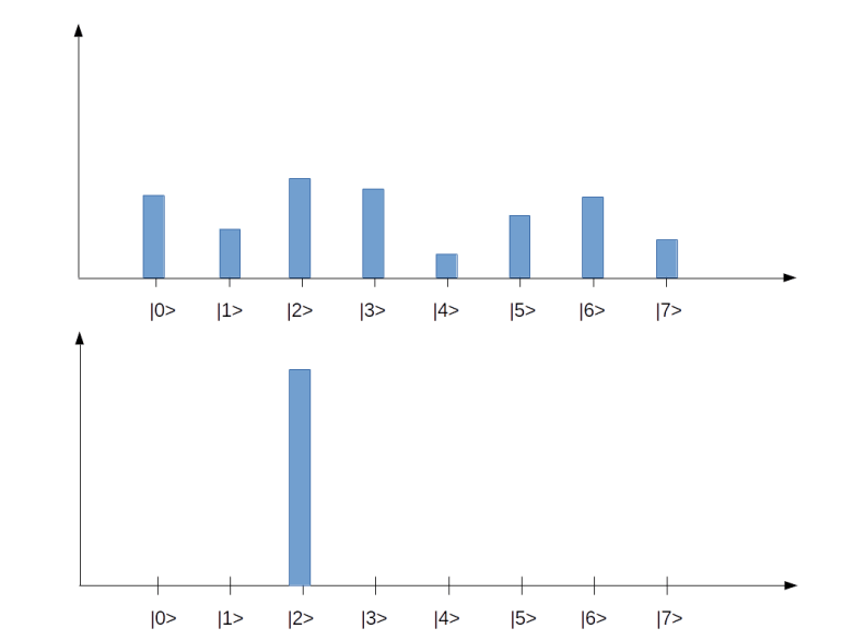
Each tick on the horizontal axis represents one of the basis states $|i \rangle$ . In our example, we have eight basis states, corresponding to a quantum system with 3 qubits. The bar represents the amplitude, i.e. the number $a_i$ in the superposition above (of course this is only a very incomplete representation, as it represents the amplitudes as real numbers, whereas in reality they are complex numbers). The upper state in the diagram represents a superposition for which all of the amplitudes are different from zero. The second diagram represents a state in which all but one amplitude is zero, i.e. a state that is equivalent to one of the basis vectors ( $|2\rangle$ in this case). These states correspond to the eight states of a corresponding classical system with three bits, whereas all states with more than one bar are true superpositions which have no direct equivalent in the classical case. We will later see how similar diagrams can be used to visualize the inner workings of simple quantum algorithms.

Qubits are nice, but in order to perform computations, we have to manipulate them somehow. This is done using quantum gates which I will discuss in my next post.

The EM algorithm and Gaussian mixture models – part II

In this post, I will discuss the general form of the EM algorithm to obtain a maximum likelihood estimator for a model with latent variables.

First, let us describe our model. We suppose that we are given some joint distribution of a random variable X (the observed variables) and and random variable Z (the latent variables) and are interested in maximizing the likelihood of an observed sample x of the visible variable X. We also assume that the joint distribution depends on a parameter $\Theta$ , in practice this could be weights, bias terms or any other parameters. To simplify things a bit, we will also assume that the latent variable is finite. Our aim is to maximize the log likelihood, which we can – under these assumptions – express as follows.

$\ln P(x |\Theta) = \ln \sum_z P(x,z | \Theta)$

Even if the joint distribution belongs to some exponential family, the fact that we need to consider the logarithm of the sum and not the sum of the logarithms makes this expression and its gradient difficult to calculate. So let us look for a different approach.

To do this, let us assume that we are given a value $\Theta$ of the parameter and let us try to understand how the likelihood changes if we pass from $\Theta$ to some other value $\Theta'$ . For that purpose, we introduce a term that is traditionally called Q and defined as follows (all this is a bit abstract, but will become clearer later when we do an example):

$Q(\Theta'; \Theta) = E \left[ \ln P(x,z | \Theta') | x, \Theta \right]$

That looks a bit complicated, so let me explain the notation a bit. We want to define a function Q that will be a function of the new parameter value $\Theta'$ . This function will, in addition, depend on the current value $\Theta$ which we consider as a parameter.

The right hand side is an expectation value. In fact, for each value of the visible variable x and the parameter $\Theta$ , we have a probability distribution on the space in which Z lives, given by the conditional probability of Z given x and $\Theta$ . Whenever we have a function depending on z, we can therefore form the expectation value as usual, i.e. as the weighted sum over all function values, weighted by the probability of z. In particular, we can do this for the function $\ln P(x,z | \Theta')$ of z. Thus the right hand side is, spelled out

$E \left[ \ln P(x,z | \Theta') | x, \Theta \right] = \sum_z \ln P(x,z | \Theta') P(z | x, \Theta)$

That is now again a sum of logarithms, not a logarithm of a sum, and we can hope to be able to deal with this much better.

This is nice, but so far we have only introduced a rather complicated additional object – what do we gain? It turns out that essentially, maxizing Q will effectively maximize the likelihood. Let us make this bold statement a bit more precise. Suppose we are able to iteratively maximize Q. Expressed formally, this would mean that we are able to find a sequence $\Theta^0, \Theta^1, \dots$ of parameters such that when passing from $\Theta^t$ to $\Theta^{t+1}$ , the value of Q does not decrease, i.e.

$Q(\Theta^{(t+1)};\Theta^{(t)}) \geq Q(\Theta^{(t)} ; \Theta^{(t)})$

Then this very same sequence will be a sequence of parameters for which the log-likelihood is non-decreasing as well, i.e.

$\ln P(x | \Theta^{(t+1)}) \geq \ln P(x | \Theta^{(t)})$

I will not include a proof for this in this post (the proof identifies the difference between any two subsequent steps as a Kullback-Leibler divergence and makes use of the fact that a Kullback-Leibler divergence is never negative, you can find a a proof in the references, in particular in [2], or in my more detailed notes on the EM algorithm and Gaussian mixture models, where I also briefly touch on convergence). Instead, let us try to understand how this can be used in practice.

Suppose that we have already constructed some parameter $\Theta^t$ . The algorithm then proceeds in two steps. First, we calculate Q as a function of the new parameter $\Theta^{t+1}$ . As Q is defined as an expectation value, this step is called the expectation step. Once we have that, we try to maximize Q, i.e. we try to find a value for the parameter $\Theta^{t+1}$ such that $Q(\Theta^{t+1}; \Theta^t)$ is maximized. This part of the algorithm is therefore called the maximization step. 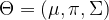Then we start over, using $\Theta^{t+1}$ as new starting point. Thus the algorithm alternates between an expectation and a maximization step, leading to the name EM algorithm.

To see how this works in practice, let us now return to our original example – Gaussian mixtures. Here the parameter $\Theta$ is given by

$\Theta = (\mu, \pi, \Sigma)$

We consider a random variable X which has N components, each of which being a vector X_n in a d-dimensional space and corresponding to one sample vector (so in the language of machine learning, N will be our batch size). Similarly, Z consists of N components z_n which again are subject to the restriction that only one of the z_nk be different from zero. We assume that the joint representation of our model is given by

$P(x , z) = \prod_n \prod_k \pi_k^{z_{nk}}{\mathcal N} (x_n, \mu_k , \Sigma_k)^{z_{nk}}$

Now we need to compute Q. The calculation is a bit lengthy, and I will skip most of it here (you can find the details in the references or my notes for this post). To state the result, we have to introduce a quantity called responsibility which is defined as follows.

$r_{nk} = \frac{\pi_k {\mathcal N}(x_n ; \mu_k, \Sigma_k)} {\sum_{j} \pi_j {\mathcal N}(x_n ; \mu_j, \Sigma_j) }$

From this definition, is it clear that the responsibility is always between zero and one, and in fact is has an interpretation of a (conditional) probability that sample n belongs to cluster k. Note that the responsibility is a function of the model parameters $\mu, \pi$ and $\Sigma$ . Using this notation, we can now write down the result of calculating the Q function:

$Q(\Theta'; \Theta) = \sum_n \sum_k r_{nk} \ln \pi'_k + \sum_n \sum_k r_{nk} \ln {\mathcal N}(x ; \mu'_k, \Sigma'_k)$

where the responsibilities are calculated using the old parameter set $\Theta = (\mu, \pi, \Sigma)$ . For a fixed $\Theta$ , this is a function of the new parameters $\mu', \pi'$ and $\Sigma'$ , and we can now try to maximize this function with respect to these parameters. This calculation is not difficult, but again a bit tiresome (and requires the use of Lagrangian multipliers as there is a constraint on the $\pi_k$ ), and I again refer to my notes for the details. When the dust settles, we obtain three simple expressions. First, the new values for the cluster means are given by

$\mu'_k = \frac{\sum_n r_{nk} x_n}{\sum_n r_{nk}}$

This starts to look familiar – this is the same expression that we did obtain for the cluster centers for the k-means algorithm! In fact, if we arrange the r_nk as a matrix, the denominator is the sum across column k and the numerators is the weighted sum over all data points. However, there is one important difference – it is no longer true that given n, only one of the r_nk will be different from one. Instead, the r_nk are soft assignments that model the probability that the data point x_n belongs to cluster k.

To write down the expression for the new value of the covariance matrix, we again need a notation first. Set

$N_k = \sum_n r_{nk}$

which can be interpreted as the number of soft assignments of points to cluster k. With that notation, the new value for the covariance matrix is

$\Sigma'_k = \frac{1}{N_k} \sum_n r_{nk} (x_n - {\mu'}_k)(x_n - {\mu'}_k)^T$

Finally, we can use the method of Lagrange multipliers to maximize with respect to the weights $\pi_k$ (which always need to sum up to one), and again obtain a rather simple expression for the new value.

$\pi'_k = \frac{N_k}{N}$

Again, this is intuitively very appealing – the probability to be in cluster k is updated to be the number of points with a soft assignment to k divided by the total number of assignments

We now have all the ingredients in place to apply the algorithm in practice. Let us summarize how this will work. First, we start with some initial value for the parameters – the weights $\pi$ , the covariance matrices $\Sigma_k$ and the means $\mu_k$ – which could, for instance, be chosen randomly. Then, we calculate the responsibilities as above – essentially, this is the expectation step, as it amounts to finding Q.

In the M-step, we then use these responsibilities and the formulas above to calculate the new values of the weights, the means and the covariance matrix. This involves a few matrix operations, which can be nicely expressed by the operations provide by the numpy library.

In the example above, we have created two sets of 500 sample points from different Gaussian mixture distributions and then applied the k-means algorithm and the EM algorithm. In the top row, we see the results of running the k-means algorithm. The color indicates the result of the algorithm, the shape of the marker indicates the original cluster to which the point belongs. The bottom row displays the results of the EM algorithm, using the same pattern.

We see that while the first sample (diagrams on the left) can be clustered equally well by both algorithms, the k-means algorithm is not able to properly cluster the second sample (diagrams on the right), while the EM algorithm is still able to assign most of the points to the correct cluster.

If you want to run this yourself, you can – as always – find the source code on GitHub. When playing with the code and the parameters, you will notice that the results can differ substantially between two consecutive runs, this is due to the random choice of the initial parameters that have a huge impact on convergence (and sometimes the code will even fail because the covariance matrix can become singular, I have not yet fixed this). Using the switch --data=Iris, you can also apply the EM algorithm to the Iris data set (you need to have a copy of the Iris data file in the current working directory) and find again that the results vary significantly with different starting points.

The EM algorithm has the advantage of being very general, and can therefore be applied to a wide range of problems and not just Gaussian mixture models. A nice example is the Baum Welch algorithm for training Hidden Markov models which is actually an instance of the EM algorithm. The EM algorithm can even be applied to classical multi-layer feed forward networks, treating the hidden units as latent variables, see [3] for an overview and some results. So clearly this algorithm should be part of every Data Scientists toolbox.

References

1. C.M. Bishop, Pattern recognition and machine learning, Springer, New York 2006
2. A.P. Dempster, N.M. Laird, D.B. Rubin, Maximum likelihood from incomplete data via the EM-algorithm, Journ. Royal Stat. Soc. Series B. Vol. 39 No. 1 (1977), pp. 1-38
3. Shu-Kay Ng, G.J. McLachlan, Using the EM Algorithm to Train Neural Networks: Misconceptions and a New Algorithm for Multiclass Classification, IEEE Transaction on Neural Networks, Vol. 15, No. 3, May 2004

The EM algorithm and Gaussian mixture models – part I

In the last few posts on machine learning, we have looked in detail at restricted Boltzmann machines. RBMs are a prime example for unsupervised learning – they learn a given distribution and are able to extract features from a data set, without the need to label the data upfront.

However, there are of course many other, by now almost classical, algorithms for unsupervised learning. In this and the following posts, I will explain one of the most commonly applied algorithms in this field, namely the EM algorithm.

As a preparation, let us start with a very fundamental exercise – clustering. So suppose that we are given a data set which we suspect to consist of K clusters. We want to identify these clusters, i.e. to each point in the dataset, we want to assign the number of the cluster to which the point belongs.

More precisely, let us suppose that we are given a set ${\mathcal D} = \{ x_i, \dots, x_N\}$ of points in some euclidian space and a number K of clusters. We want to identify the centre $\mu_i$ of each cluster and then assign the data points x_i to some of the $\mu_j$ , namely to the $\mu_j$ which is closest to x_i. We can encode the assignment of data points to clusters in a matrix R_ij where R_ij = 1 if data point x_i belongs to cluster j with centre $\mu_j$ . Thus each row of R corresponds to a data point and is non-zero in exactly one column, where it is one. This is known as 1-of-K encoding.

For each value of i, the squared distance of x_i to the centre of the cluster to which it is assigned is then given by

$\sum_j R_{ij} \| x_i - \mu_j |^2$

where we note that only one of the summands is different from zero. Assigning the data points to the clusters and positioning the centre points of the clusters then amounts to minimizing the loss function

$l(\mu, R) = \sum_i \sum_j R_{ij} \langle x_i - \mu_j , x_i - \mu_j \rangle$

where the brackets denote the usual euclidean scalar product.

Now let us see how we can optimize this function. For a fixed vector $\mu$ of cluster centers, we can easily minimize R_ij by assigning each data point to the cluster whose center is closest to x_i. Thus we set

$R_{ij} = \begin{cases} 1 & \text{if} \, j = \arg \min \| x_i - \mu_j \|^2 \\ 0 & \text{otherwise} \end{cases}$

Conversely, given a matrix R which we hold fixed, it is likewise easy to minimize $\mu_j$ . As there are no further constraints on $\mu_j$ , we can find the minimum by differentiating the loss function. We find that the derivative is zero if and only if

$0 = \sum_i R_{ij}(x_i - \mu_j)$

holds for all j. Assuming for a moment that each cluster has at least one data point assigned to it, i.e. that none of the columns of R contains zeroes only, we can solve this by

$\mu_j = \frac{\sum_i x_i R_{ij}}{\sum_i R_{ij}}$

which is also easily seen to be a local minimum by taking the second derivative.

Note that this term has an obvious geometric interpretation. The denominator in this expression is the number of data points that are currently assigned to cluster j. The numerator is the sum of all data points assigned to this cluster. Thus the minimum is the mean value of the positions of the data points that are currently assigned to the cluster (a physicist would call this the center of gravity of the cluster). This is the reason why this method is called the k-means algorithm. If no data points are assigned to the cluster, the loss function does not depend on $\mu_j$ and we can choose any value that we want.

The algorithm now works as follows. First, we choose centers $\mu_j$ at will – it is common to use some of the data points for this purpose. Then we assign each data point to a center using the formula for R_ij derived above. We then adjust the center points $\mu_j$ and reallocate the points to the new centers and so forth.

From our discussion above, it is clear that each full iteration of this procedure will reduce the loss function. This does of course not imply that the algorithm converges to a global minimum, as it might get stuck in local minima or saddle points. In practice, the algorithm is executed until the cluster assignments and centers do not change any more substantially or for a given number of steps.

The diagram above shows the result of applying this algorithm to a set of points that is organized in two clusters. To generate the data, 100 samples were drawn from 2-dimensional Gaussian distributions. On the left hand side, half of the the samples were centered at the point (5,1), the other samples at (1,4), and both had standard deviation 0.6. On the right hand side, the same centers were used, but only a small number of samples were drawn from the second distribution which had standard deviation 0.5, whereas most samples came from the first distribution with standard deviation 0.8. Then 10 iterations of the k-means algorithm were applied to the resulting sample set. The points in the sample were then plotted with a color indicating the assignment to clusters resulting from the matrix R. The actual cluster from which the sample was drawn is indicated by the shape – a point is cluster one, a diamond is cluster two.

We see that in the example on the left hand side, the algorithm has correctly assigned all points to their original cluster. For the example on the right hand side, the situation is different – the algorithm did actually assign significantly more points to the blue cluster, i.e. there are many wrong assignments (blue points). This does not change substantially if we increase the number of iterations, even with 100 iterations, we still see many wrong assigments for this example. If you want to reproduce the example and play a bit with the parameters, you can get the sourcecode for a straightforward implementation in Python from my GitHub repository.

The K-means algorithm is very simple and straightforward, but seems to have limitations because it cannot determine the shape of a distribution, only its center. It turns out that K-means is a special case of a broader class of algorithms that we now study, hoping to find more robust algorithms.

In our example, we have generated sample data as a combination of two Gaussian distributions. What if we just change the game and simply assume that our data is of this type? In other words, we assume an underlying probabilistic model for our sample data. Once we have that, we can pull all the tricks that statistical inference can offer – we can calculate maximum likelihood and maximum posterior probability, we can try to determine the posterior or even sample from the model.

Thus let us try to fit our data to a model of the form

$P(x) = \sum_k \pi_k {\mathcal N}(x ; \mu_k, \Sigma_k)$

where ${\mathcal N}(x ; \mu_k, \Sigma_k)$ is a multivariate Gaussian distribution with mean $\mu_k$ and covariance matrix $\Sigma_k$ , i.e.

${\mathcal N}(x ; \mu_k, \Sigma_k) = \frac{1}{\sqrt{(2\pi)^d \det(\Sigma)}} \exp (-\frac{1}{2} \langle x - \mu_k, \Sigma_k^{-1}(x - \mu_k)\rangle)$

and the $\pi_k$ are non-negative real numbers with $\sum_k \pi_k = 1$ .

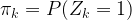
Let us now see how this equation looks like if we use a 1-of-K encoding. We introduce a random variable Z that takes values in $\{ 0, 1\}^K$ with the additional constraint that only one of the Z_k is allowed to be different from zero. We interpret $\pi_k$ as the probability

$\pi_k = P(Z_k = 1)$

Then

$P(Z = z) = \prod_k \pi_k ^{z_k}$

and we can write

$P(X=x) = \sum_z P(Z=z) P(X=x | Z=z) = \sum_z P(x,z)$

where $P(z)$ is as above and

$P(X = x | Z = z) = \prod_k {\mathcal N}(x ; \mu_k, \Sigma_k)^{z_k}$

This is a very general type of distribution which reflects a common pattern in machine learning, namely the introduction of so called latent or hidden variables. In general, latent or hidden variables are random variables that are a part of the model which cannot be observed, i.e. are not part of the input or the output of the model. We have seen latent variables in action several times – adding hidden units to a neural network introduces latent variables and makes the model much more powerful, the hidden layer of a restricted Boltzmann machine serves as memory to learn features, and latent variables that are used to construct a mixture of Gaussians as above allow us to model a much broader class of distributions than a model with just one Gaussian.

Intuitively, it is also clear how to sample from such a model. In a first step, we sample from Z, in other words we determine the index k randomly according to the distribution given by the $\pi_k$ . Once we have k, we then sample from the conditional distribution $P(X = x | Z = z)$ . As we already have k, this amounts to sampling from the Gaussian distribution ${\mathcal N}(x ; \mu_k, \Sigma_k)$ with mean $\mu_k$ and covariance matrix $\Sigma_k$ .

In the example above, we have first applied this procedure to a one-dimensional Gaussian mixture with K=2. The histogram shows the result of the sampling procedure, the solid lines are the probability density functions of the two individual Gaussian distributions, multiplied by the respective weight. On the right hand side, the result of sampling a Gaussian mixture in two dimensions is displayed (you can download the notebook used to produce this example here).

When we now try to fit this model to the sample data, we again have to calculate the likelihood function and try to maximize it. However, it turns out that the gradient of the likelihood is not so easy to calculate, and it might very well be that there is no closed form solution or that we obtain rather complicated expressions for the gradient. Fortunately, there is an alternative that works for very general models and does not require knowledge of the gradient – the EM algorithm. In the next post, I will present the algorithm in this general setup, before we apply it to our original problem and compare the results with the k-means algorithm.

References

Why you need statistics to understand neuronal networks

When I tried to learn about neuronal networks first, I did what probably most of us would do – I started to look for tutorials, blogs etc. on the web and was surprised by the vast amount of resources that I found. Almost every blog or webpage about neuronal networks has a section on training a simple neuronal network, maybe on the MNIST data set, using a framework like TensorFlow, Theano or MXNET. When you follow such a tutorial, a network is presented as a collection of units and weights. You see how the output of the network is calculated and then an error function – sometimes least squares, sometimes something else – is presented. Often, a regulation term is applied, and then you are being told that the automatic gradient calculation features of the framework will do the gradient descent algorithm for you and you just have to decide on an optimizer and run the network and enjoy the results.

Sooner or later, however, you will maybe start to ask a few questions. Why that particular choice of the loss function? Where does the regulator come from? What is a good initial value for the weights and why? Where does the sigmoid function come from? And many, many other questions….

If you then decide to dig deeper, using one of the many excellent textbooks or even try to read some of the original research papers (and some are actually quite readable), you will very soon be confronted with terms like entropy, maximum likelihood, posterior distribution, Gaussian mixtures and so on, and you will realize that the mathematics of neuronal networks has a strong overlap with mathematical statistics. But why? Why is that a good language to discuss neuronal networks, and why should you take the time to refresh your statistics knowledge if you really want to understand neuronal networks? In this post, I will try to argue that statistical inference comes up very naturally when you try to study neuronal networks.

Many neuronal networks are designed to excel at classification tasks. As an example, suppose you wanted to design and train a neuronal network that, given data about an animal, classifies the animal as either a bird or some other animal (called a “non-bird” for convenience). So our starting point is a set modelling all possible objects that could be presented to the network. How exactly we model this set is not so important, more important is that in general, the network will not have access to all the data about the animal, but only to certain attributes of elements in the set called features. So there could be a feature which we call X₁ and which is defined as

$X_1 = \text{the animal can fly}$

taking values in $\{0,1\}$ . Another data point the network could get is

$X_2 = \text{length of animal in cm}$

taking values in the reals and so forth. More generally, we assume that on the set of all possible objects, we have certain functions X_i taking values in, say, the real numbers. Based on these numbers, the network will then try to take a decision whether a given animal is a bird or not. Thus we do not have to deal directly with our space of objects, but use the functions X_i as primary objects.

If the network had a chance to look at every possible animal, this would be easy, even though it would cost a lot memory – it could simply remember all possible combinations of features and for each feature, store the correct answer. In reality however, this does not work. Instead, we have access to a small subset of the data – a sample – for which we can evaluate the X_i. Based on this subset, we then have to derive a model which gives the right answer in as many cases as possible. Thus we try to make a statement about the full space of things that could be presented to our network for classification based on a small sample.

This is where probabilities come into play very naturally. We need to assume that our sample has been chosen randomly, but still we need to make assertions about the full set. This is exactly what inferential statistics is doing. The fact that our sample is chosen randomly turns our X_i into random variables. Similarly, the variable

$Y = \text{is a bird}$

taking values in $\{0,1\}$ is a random variable, and we try to gain information on the distribution of Y across the full population based on its values on a given set of labelled samples, i.e. a set of samples where Y is known. Thus Y would represent the labels or targets in the language of neuronal networks. Applying the methods of statistical inference to this situation would typically start by choosing a statistical model and than using estimators or hypothesis testing to make deductions.

Apart from the fact that we have to derive information on the full population based on a sample, there is another reason why probabilities appear naturally in the theory of machine learning. In many cases, the available input – being a reduction of the full set of data – is not sufficient to classify the sample with full certainty. To see this, let us go back to our examples. How would you derive the property “bird” from the given data “can fly” and “length”? Not all animals than can fly are birds – and not all birds can fly. So we have to try to distinguish for instance a butterfly from a hummingbird based on the length. The smallest hummingbird – a bee hummingbird – is about 5 cm in length. The largest known butterfly – the Queen’s Alexandra birdwing – can be as long as 8 cm (both informations taken from Wikipedia). Thus our data is not sufficient to clearly distinguish butterflies and birds in all cases!

However, very small birds and very large butterflies have one thing in common – they are rare. So chances are that a given animal that can fly and is larger than 5 cm is actually a bird (yes, I know, there are bats….). In other words, if again Y denotes the variable which is 1 on birds and 0 on all other animals, we can in general not hope that Y is a function of the X_i, but we can hope that given some values of the X_i, the probability $P(Y=1)$ to be a bird is a function of the X_i. In other words, using the language of conditional probabilities,

$P(Y=1 | X = x) = f(x)$

with some unknown function f. In a Bayesian interpretation of probability, the certainty with which can say “this animal is a bird” is a function of the values x_i of the observable variables X_i.

With these considerations, we now arrive at the following mathematical model for what a classification algorithm is about. We are given a probability space $(P, \Omega)$ with a vector valued random variable X. The attributes of a sample are described by the feature vector X in some subset of m-dimensional euclidian space, where m is the number of different features. In our example, m=2, as we try to classify animals based on two properties. The result of the classification is described by a random variable Y taking – for the simple case of a binary classification problem – values in $\{0,1\}$ . We then assume that

$P(Y =1 | X=x) = f(x;w_0)$

where $f(\cdot;w)$ is a function parametrized by some parameter w that we call the weights of the model. The actual value w₀ of w is unknown. Based on a sample for X and Y, we then try to fit the model, i.e. we try to find a value for w such that $f(\cdot, w)$ models the actual conditional distribution of Y as good as possible. Once the fitting phase is completed, we can then use the model to derive predictions about objects which are not in our initial sample set.

This model sounds a bit abstract, but many feed forward neuronal networks can be described with this or similar models. And we can now apply the full machinery of mathematical statistics – we can calculate cross entropies and maximum likelihood, we can analyse converge and variance, we can apply the framework of Bayesian statistics and Monte Carlo methods. This is the reason why statistics is so essential when it comes to describing and analyzing neuronal networks. So on the next rainy Sunday afternoon, you might want to grab a steaming hot cup of coffee, head towards your arm chair and spent some time with one of the many good exposures on this topic, like chapter IV in MacKays book on Machine Learning, or Bishops “Pattern recognition and machine learning” or chapter 3 of the deep learning book by Goodfellow, Bengio and Courville.

The Metropolis-Hastings algorithm

In this post, we will investigate the Metropolis-Hastings algorithm, which is still one of the most popular algorithms in the field of Markov chain Monte Carlo methods, even though its first appearence (see [1]) happened in 1953, more than 60 years in the past. It does for instance appear on the CiSe top ten list of the most important algorithms of the 20th century (I got this and the link from this post on WordPress).

Before we get into the algorithm, let us once more state the problem that the algorithm is trying to solve. Suppose you are given a probability distribution $\pi$ on some state space X (most often this will be a real euclidian space on which you can do floating point arithmetic). You might want to imagine the state space as describing possible states of a physical system, like spin configurations in a ferromagnetic medium similar to what we looked at in my post on the Ising model. The distribution $\pi$ then describes the probability for the system to be in a specific state. You then have some quantity, given as a function f on the state space. Theoretically, this is a quantity that you can calculate for each individual state. In most applications, however, you will never be able to observe an individual state. Instead, you will observe an average, weighted by the probability of occurence. In other words, you observe the expectation value

$\langle f \rangle = \int_X f d\pi$

of the quantity f. Thus to make a prediction that can be verified or falsified by an observation, you will have to calculate integrals of this type.

Now, in practice, this can be very hard. One issue is that in order to naively calculate the integral, you would have to transverse the entire state space, which is not feasible for most realistic problems as this tends to be a very high dimensional space. Closely related to this is a second problem. Remember, for instance, that a typical distribution like the Boltzmann distribution is given by

$\pi(x) = \frac{1}{Z} e^{-\beta E(x)}$

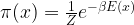
The term in the numerator is comparatively easy to calculate. However, the term in the denominator is the partition function, and is itself an integral over the state space! This makes even the calculation of $\pi(x)$ for a single point in the state space intractable.

But there is hope – even though calculating the values of $\pi$ for one point might be impossible, in a distribution like this, calculating ratios of probabilities is easy, as the partition function cancels out and we are left with the exponential of an energy difference! The Metropolis-Hasting algorithm leverages this and also solves our state space problem by using a Markov chain to approximate the integral. So the idea is to build a Markov chain X_t that converges and has $\pi$ as an invariant distribution, so that we can approximate the integral by

$\langle f \rangle = \int_X f d\pi \approx \frac{1}{N} \sum_{t=1}^N f(X_t)$

for large values of N.

But how do we construct a Markov chain that converges to a given distribution? The Metropolis Hastings approach to solve this works as follows.

The first thing that we do is to choose a proposal density q on our state space X, i.e. a measurable function

$q \colon X \times X \rightarrow [0,\infty)$

such that for each x, $\int q(x,y) dy = 1$ .

Then q defines a Markov chain, where the probability to transition into a measurable set A being at a point x is given by the integral

$Q(x,A) = \int_{\mathcal X} q(x,y) dy$

Of course this is not yet the Markov chain that we want – it has nothing to do with $\pi$ , so there is no reason it should converge to $\pi$ . To fix this, we now adjust the kernel to incorporate the behaviour of $\pi$ . For that purpose, define

$\alpha(x,y) = \begin{cases} \min \{ 1, \frac{\pi(y)q(y,x)}{\pi(x)q(x,y)} \} & \text{if } \pi(x) q(x,y) > 0 \\ 1 & \text{if } \pi(x) q(x,y) = 0 \end{cases}$

This number is called the acceptance probability, and, as promised, it only contains ratios of probabilities, so that factors like the partition function cancel and do not have to be computed.

The Metropolis Hastings algorithm now proceeds as follows. We start with some arbitrary point x₀. When the chain has arrived at x_n, we first draw a candidate y for the next location from the proposal distribution $q(x_n, \cdot)$ . We now calculate $\alpha$ according to the formula above. We then accept the proposal with probability $\alpha$ , i.e. we draw a random sample U from a uniform distribution and accept if $U \leq \alpha$ . If the proposal is accepted, we set x_n+1 = y, otherwise we set x_n+1 = x_n, i.e. we stay where we are.

Clearly, the x_n are samples from a Markov chain, as the position at step x_n only depends on the position at step x_n-1. But is still appears to be a bit mysterious why this should work. To shed light on this, let us consider a case where the expressions above simplify a bit. So let us assume that the proposal density q is symmetric, i.e. that

$q(x,y) = q(y, x)$

This is the original Metropolis algorithm as proposed in [1]. If we also assume that $\pi$ and q are nowhere zero, the acceptance probability simplifies to

$\alpha(x,y) = \min \{ 1, \frac{\pi(y)}{\pi(x)} \}$

Thus we accept the proposal if $\pi(y) \geq \pi(x)$ with probability one. This is very similar to a random search for a global maximum – we start at some point x, choose a candidate for a point with higher value of $\pi$ at random and proceed to this point. The major difference is that we also accept candidates with $\pi(y) < \pi(x)$ with a non-zero probability. This allows the algorithm to escape a local maximum much better. 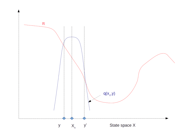Intuitively, the algorithm will still try to spend more time in regions with large values of $\pi$ , as we would expect from an attempt to sample from the distribution $\pi$ .

The image above illustrates this procedure. The red graph displays the distribution $\pi$ . If our algorithm is currently at step x_n, the purpose is to move “up-hill”, i.e. to the left in our example. If we draw a point like y from q which goes already in the right directory, we will always accept this proposal and move to y. If, however, we draw a point like y’, at which $\pi$ is smaller, we would accept this point with a non-zero probability. Thus if we have reached a local maximum like the one on the right hand side of the diagram, there is still a chance that we can escape from there and move towards the real maximum to the left.

In this form, the algorithm is extremely easy to implement. All we need is a function propose that creates the next proposal, and a function p that calculates the value of the probability density $\pi$ at some point. Then an implementation in Python is as follows.

import numpy as np
chain = []
X = 0
chain.append(X)
for n in range(args.steps):
  Y = propose(X)
  U = np.random.uniform()
  alpha = p(Y) / p(X)
  if (U <= alpha):
    X = Y
  chain.append(X)

In the diagram below, this algorithm has been applied to a Cauchy distribution with mode zero and scale one, using a normal distribution with mean x and standard deviation 0.5 as a proposal for the next location. The chain was calculated for 500.000 steps. The diagram in the upper part shows the values of the chain during the simulation.

Then the first 100.000 steps were discarded and considered as "burn-in" time for the chain to stabilize. Out of the remaining 400.000 sample points, points where chosen with a distance of 500 time steps to obtain a sample which is approximately independent and identically distributed. This is called subsampling and typically not necessary for Monte Carlo integration (see [2], chapter 1 for a short discussion of the need of subsampling), but is done here for the sake of illustration. The resulting subsample is plotted as a histogramm in the lower left corner of the diagram. The yellow line is the actual probability density.

We see that after a few thousand steps, the chain converges, but continues to have spikes. However, the sampled distribution is very close to the sample generated by the Python standard method (which is to take the quotient of two independent samples from a standard normal distribution).

In the diagram at the bottom, I have displayed how the integral of two functions ( $\sin(x)$ and $\cos(x)$ ) approximated using the partial sums develops over time. We see that even though we still have huge spikes, the integral remains comparatively stable and converges already after a few thousand iterations. Even if we run the simulation only for 1000 steps, we already get close to the actual values zero (for $\sin(x)$ for symmetry reasons) and $\approx 0.3678$ (for $\cos(x)$ , obtained using the scipy.integrate.quad integration routine).

In the second diagram in the middle row, I have plotted the autocorrelation versus the lag, as an indicator for the failure of the sample points to be independent. Recall that for two samples X and Y, the Pearson correlation coefficient is the number

$\frac{E((X-\bar{X})(Y-\bar{(Y)})}{\sigma_X \sigma_Y}$

where $\sigma_X$ and $\sigma_Y$ are the standard deviations of X and Y. In our case, given a lag, i.e. a number l less than the length of the chain, we can form two samples, one consisting of the points $X_0, X_2, \dots$ and the second one consisting of the points of the shifted series $X_l, X_{l+1}, X_{l+2}, \dots$ . The autocorrelation with lag l is then defined to be the correlation coefficient between these two series. In the diagram, we can see how the autocorrelation depends on the lag. We see that for a large lag, the autocorrelation becomes small, supporting our intuition that the series and the shifted series become independent. However, if we execute several simulation runs, we will also find that in some cases, the convergence of the autocorrelation is very slow, so care needs to be taken when trying to obtain a nearly independent sample from the chain.

In practice, the autocorrelation is probably not a good measure for the convergence of a Markov chain. It is important to keep in mind that obtaining an independent sample is not the point of the Markov chain – the real point is that even though the sample is autocorrelated, we can approximate expectation values fairly well. However, I have included the autocorrelation here for the sake of illustration.

This form of proposal distributions is not the only one that is commonly used. Another choice that appears often is called an independence sampler. Here the proposal distribution is chosen to be independent of the current location x of the chain. This gives us an algorithm that resembles the importance sampling method and also shares some of the difficulties associated with it – in my notes on Markov chain Monte Carlo methods, I have included a short discussion and a few examples. These notes also contain further references and a short discussion of why and when the Markov chain underlying a Metropolis-Hastings sampler converges.

Other variants of the algorithm work by updating – in a high-dimensional space – either only one variable at a time or entire blocks of variables that are known to be independent.

Finally, if we are dealing with a state space that can be split as a product $X_1 \times X_2$ , we can use the conditional probability given either x₁ or x₂ as a proposal distribution. Thus, we first fix x₂, and draw a new value for x₁ from the conditional probability for x₁ given the current value of x₂. Then we move to this new coordinate, fix x₁, draw from the conditional distribution of x₂ given x₁ and set the new value of x₂ accordingly. It can be shown (see for example [5]) that the acceptance probability is one in this case. So we end up with the Gibbs sampling algorithm that we have already used in the previous post on Ising models.

Monte Carlo sampling methods are a broad field, and even though this has already been a long post, we have only scratched the surface. I invite you to consult some of the references below and / or my notes for more details. As always, you will also find the sample code on GitHub and might want to play with this to reproduce the examples above and see how different settings impact the result.

In a certain sense, this post is the last post in the series on restricted Boltzmann machines, as it provides (at least some of) the mathematical background behind the Gibbs sampling approach that we used there. Boltzmann machines are examples for stochastic neuronal networks that can be applied to unsupervised learning, i.e. the allow a model to learn from a sample distribution without the need for labeled data. In the next few posts on machine learning, I will take a closer look at some other algorithms that can be used for unsupervised learning.

References

1. N. Metropolis,A.W. Rosenbluth, M.N. Rosenbluth, A.H. Teller, E. Teller, Equation of state calculation by fast computing machines, J. Chem. Phys. Vol. 21, No. 6 (1953), pp. 1087-1092
2. S. Brooks, A. Gelman, C.L. Jones,X.L. Meng (ed.), Handbook of Markov chain Monte Carlo, Chapman Hall / CRC Press, Boca Raton 2011
3. W.K. Hastings, Monte Carlo sampling methods using Markov chains and their applications, Biometrika, Vol. 57 No. 1 (1970), pp. 97-109
R.M. Neal, Probabilistic inference using Markov chain Monte Carlo methods, Technical Report CRG-TR-93-1, Department of Computer Science, University of Toronto, 1993
5. C.P. Robert, G. Casella, Monte Carlo Statistical Methods,
Springer, New York 1999

Recurrent and ergodic Markov chains

Today, we will look in more detail into convergence of Markov chains – what does it actually mean and how can we tell, given the transition matrix of a Markov chain on a finite state space, whether it actually converges.

So suppose that we are given a Markov chain on a finite state space, with transition probabilities described by a matrix K as in the previous post on this topic.

We have seen that the distribution of X_n is given by $\mu K^n$ where $\mu$ is the initial distribution. So if Kⁿ converges, we can expect the distribution of X_n to converge as well. If there is a matrix $K^\infty$ such that

$\lim_{n \rightarrow \infty} K^n = K^\infty$

then of course

$K^\infty K = (\lim_{n \rightarrow \infty} K^n) K = \lim_{n \rightarrow \infty} K^{n+1} = K^\infty$

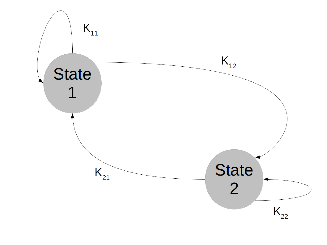
In other words, each row $\pi$ of $K^\infty$ will have the property that $\pi K = \pi$ . Interpreting K as transition probabilities, this implies that if the distribution of X_n is $\pi$ , the distribution of X_n+1 will again be $\pi$ . Any distribution, described by a row vector $\pi$ with row sum 1, for which this holds is called an invariant distribution and traditionally denoted by $\pi$ . In other words, invariant distributions correspond to eigenvectors of the transposed matrix K^T with eigenvalue 1, and our argument has shown that if $K^n$ converges to $K^\infty$ , then every row of $K^\infty$ will be an invariant distribution.

So convergence implies the existence of an invariant distribution. Let us next try to understand whether this invariant distribution is unique. There are obvious examples where this is not the case, the most trivial one being the unit matrix

$K = \begin{pmatrix} 1 & 0 \\ 0 & 1 \end{pmatrix}$

Obviously $K^n = K$ and the chain converges, but every vector with row sum one is an invariant distribution. This chain is too rigid, because in whatever state we start, we will stay in this state forever. It turns out that in order to ensure uniquess of an invariant distribution, we need a certain property that makes sure that the states can move around freely which is called irreducibility.

Intuitively, we say that a Markov chain is irreducible if any state can be reached from any other state in finitely many steps. For a finite state space, this is rather easy to formalize. A finite Markov chain is called irreducible if, given two states i and j, we can find some power n such that $K^n_{ij} > 0$ . In other words, given a row index i and a column index j, we can find a power n such that the element of Kⁿ at (i,j) is not zero. It turns out that if a chain is not irreducible, we can split the state space into smaller areas that the chain – once it has entered one of them – does not leave again and on which it is irreducible. So irreducible Markov chains are the buildings blocks of more general Markov chains, and the study of many properties of Markov chains can be reduced to the irreducible case.

Now let us assume that our chain is in fact irreducible. What else do we have to ask for to make sure that it converges? Again, let us as look at an obvious example.

$K = \begin{pmatrix} 0 & 1 \\ 1 & 0 \end{pmatrix}$

All even powers of this matrix are the unit matrix and all odd powers are K itself, so the Markov chain described by this transition matrix is clearly irreducible. However, there is still something wrong. If, for instance, we are in state 1 at the time t, then the probability to still be in state 1 at time t+1 is zero. Thus we are actually forced to move to state 2. In a certain sense, there is still an additional constraint on the the behaviour of the chain – the state space can be split in two pieces and we cycle through these pieces with every step. Such a chain is called periodic. If a chain is periodic, it is again obvious that we can think of it as two different chains, one chain given by the random variables X₀, X₂,… at even times and the other chain given by the random variables X₁, X₃, … at odd times. Thus again, there is a way to split the chain into parts.

So let us now focus on chains that are irreducible and aperiodic. Can we tell whether the chain converges? The answer is surprisingly simple and one of the most powerful results in the theory or Markov chains: every finite Markov chain which is irreducible and aperiodic converges. Thus once we have verified aperiodicity and irreducibility, we can be sure that the limit $K^\infty$ exists. We can say even more – we have seen that the rows of the limit are invariant distributions for K. However, one can show that an irreducible Markov chain can only have one invariant distribution. Thus we can conclude that all rows of the matrix $K^\infty$ are identical. In fact, they are all equal to the (unique) invariant distribution that again corresponds to an eigenvector of K^T with eigenvalue one.

This gives us two different approaches to calculating the invariant distribution and the limit $K^\infty$ . First, we can form high powers Kⁿ to approximate the limit $K^\infty$ . Or, alternatively, we can search for eigenvectors of the transposed matrix K^T with eigenvalue 1 using one of the known algorithms to calculate eigenvectors and eigenvalues.

Let us do this for the example of the random walk on a circle that we have studied earlier. For simplicity, we will use N = 4 this time. The transition matrix with p = 0.8 is

$K = \begin{pmatrix} 0.20 & 0.40 & 0.00 & 0.40 \\ 0.40 & 0.20 & 0.40 & 0.00 \\ 0.00 & 0.40 & 0.20 & 0.40 \\ 0.40 & 0.00 & 0.40 & 0.20 \\ \end{pmatrix}$

We can then easily implement both approaches in Python using the numpy library.

Sorry, something went wrong. Reload?

Sorry, we cannot display this file.

Sorry, this file is invalid so it cannot be displayed.

view raw TransitionMatrixMarkovChain.ipynb hosted with ❤ by GitHub

So we see that the approach to take the eigenvalues and eigenvectors gives us – in this case – the exact result (and a direct computation confirms that this is really an eigenvector), whereas the matrix power with n=20 gives a decent approximation. Both results confirm what we have observed visually in the last post – the distribution converges, and it does in fact converge to the uniform distribution. So roughly speaking, after sufficiently many steps, we end up everyhwere in the state space with equal probability.

So far, we have only discussed the case of a finite state space. In the general case, the situation is more complicated. First, we need a better definition of irreducibility, as on a general state space, the probability measure of a single point tends to be zero. It turns out that the solution is to define irreducibility with respect to a measure on the state space, which is called $\psi$ -irreducibility. Once we have that, we find two potential behaviours that do not show up in the finite case.

First, it might happen that even though the chain is irreducible, it does not properly cycle through the state space and revisits every point with finite probability, but – intuitively speaking – heads off to infinity. Such a chain is called transient and does not converge.

Second, even if the chain is not transient, we might be able to find an invariant distribution (a measure in this case), but this measure might not be a probability distribution as it is not finite. Chains with this property are called null recurrent.

And finally, the concept of converge needs to be made more precise, and it turns out to have a subtle dependency on the starting point which can be fixed by assuming so called Harris recurrence. But all this can be done and delivers a very similar result – a convergence theorem for a large class of chains (in this case aperiodic Harris recurrent Markov chains). If you would like to get deeper into this and also see proofs for the claims made in this post and references, I invite you to take a look at my short introduction to Markov chains.

We close this post with one remark which, however, is of crucial importance for applications. Suppose we have a convergent Markov chain X_t, and a function f on the state space. If the X_t were independent and identically distributed, we could approximate the expectation value of f as

$\int_X f(x) dP = \lim_{N \rightarrow \infty} \frac{1}{N} \sum_{i=1}^N f(X_i)$

where dP is the (common) distribution of the X_t. For Markov chains, however, we know that the X_t are not independent – the whole point of having a Markov chain is that X_t+1 does actually depend on X_t. However, in our example above, we have seen that the dependency gets trivial for large t as in this example, all entries in the transition matrix become equal in the limit.

Of course this is a special case, but it turns out that even in general, the approximation of the expectation value by averages across the sample is still possible. Intuitively, this is not so surprising at all. If the distributions $K^n$ of the $X_n$ converge to some invariant measure $\pi$ , the $X_n$ will, for large n, be approximately identically distributed, namely according to $\pi$ . Moreover, heuristically we have for large n, m and a fixed starting point s:

$P(X_{n+m}=i, X_n=j) = K^m_{ji} K^n_{sj} \approx \pi_i \pi_j$

On the other hand, this product is again approximately the product

$\pi_i \pi_j \approx P(X_{n+m}=i) P(X_n=j)$

Thus, intuitively, X_n and X_m are almost independent if n and m are large, which makes us optimistic that the law of large numbers could actually hold.

In fact, if X_t converges (again I refer to my notes for a more precise definition of convergence in this case), it turns out that the law of large numbers remains valid if we integrate f with respect to the invariant distribution $\pi$ :

$\int_X f(x) d\pi = \lim_{N \rightarrow \infty} \frac{1}{N} \sum_{i=1}^N f(X_i)$

This is extremely useful in applications, where often the primary purpose is not so much to obtain a sample, but to approximate otherwise intractable integrals! Once we have found a Markov chain that converges to the invariant distribution $\pi$ , we can calculate integrals over $\pi$ by running a long Markov chain until converge and then taking the average value of the function that we want to integrate for a large number of subsequent points from this chain. In fact, this is how most applications work – and this is more or less what we also did when we applied Markov chains to the problem of calculating gradients in the PCD algorithm, where this chain is given by the state of the negative particles in subsequent iterations.

So given a distribution $\pi$ , we are now lead to the question how we can possibly find a Markov chain for which this distribution is invariant and which converges. The most general answer to this question is a class of algorithms known as Metropolis-Hastings algorithms which we study in the next post in this series.

Finite Markov chains

In this post, we will look in more detail into an important class of Markov chains – Markov chains on finite state spaces. Many of the subtleties that are present when studying Markov chains in general state spaces do not appear in the finite case, while most of the key ideas and features of Markov chains are still visible, so this is a good starting point if you want to grasp the key points.

So let us assume that our state space X is finite. For simplicity, we label our states as $\{1, 2, \cdots N \}$ where N is the number of states. We also assume that all our points are measurable, i.e we consider our state space as a discrete probability space.

Now consider a sequence of random variables X₀, X₁, …. How can we formalize the idea that X_t+1 depends on X_t in a randomized way?

As so often in probability theory, let us model the dependency as a conditional probability. The conditional probability for X_t+1 to take on a value i given X_t

$P(X_{t+1} = i | X_t)$

considered as a function of X_t will assign a conditional probability to each of the states i and for each value of X_t. Therefore we can write this as a matrix

$P(X_{t+1} = i | X_t = j) = K_{ji}$

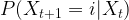
To obtain a time homogeneous Markov chain, we also assume that the matrix K does not depend on the time t. Therefore we define a Markov chain on X to be a sequence $\{X_t\}_t$ of random variables taking values in X with the Markov property saying that for all times t, the conditional distribution for X_t+1 given all previous values $X_0, X_1, \dots, X_t$ only depends on X_t, i.e.

$P(X_{t+1} | X_t, X_{t-1}, \cdots ) = P(X_{t+1} | X_t)$

We also require that this conditional probability is independent of t and is therefore given by a matrix K as in the formula above.

Markov chains on finite state spaces are often visualized as a graph. Suppose, for instance, that our state space contains only two elements: $X = \{ 1 , 2\}$ . We can think of the combined values $X_t$ for all times t as a history of states or as a random walk in the state space. The Markov property then means that the probability to transition into a next state does not depend on the full history, but only on the current state – Markov chains do not have a memory.

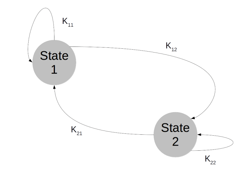
In our state space with two elements only, the Markov chain is then described by four transition probabilities: the probability to stay in state 1 when the chain is in state 1, the probability to move to state 2 when being in state 1, the probability to stay in state 2 and the probability to move to state 1 after being in state 2. This can be visualized as follows.

Let us now calculate a few probabilities to get an idea for the relevant quantities in such a model. First, suppose that at time 0, the model is in state j with probability $\mu_j$ . What is the probability to be in state j after one step? Of course we can write

$P(X_1 = i) = \sum_j P(X_1 = i, X_0 = j)$

Now, according to the rules of conditional probabilities, we can express the joint probability as follows.

$P(X_1 = i, X_0 = j) = P(X_1 = i | X_0 = j) P(X_0 = j)$

Plugging this into our previous expression and using the definitions of K and $\pi$ , we now obtain

$P(X_1 = i) = \sum_j K_{ji} \mu_j$

Thus if we think of $\mu$ as a row vector, then the probability after one step is described by the matrix product $\mu K$ .

Now let us calculate a slightly different quantity. Assume that we know that a chain starts at j. What is the probability to be at i after two steps? Using once more the rules of conditional probability and the Markov property, we can write

$P(X_2=i | X_0=j) = \sum_k P(X_2=i | X_1=k)P(X_1=k | X_0=j)$

Intuitively, this is very appealing. To get from j to i in two steps, we can take the way via any intermediate state k. To get the total probability, we simply sum up all these different probabilities! If you have ever seen path integrals in quantum mechanics, this idea will look familiar.

Again, we can write this in matrix notation. Each of the conditional probabilities on the right hand side of the expression above is a matrix element, and we find that

$P(X_2 = i | X_0 = j) = \sum_k K_{ki} K_{jk}$

so that the probability to get in two steps from j to i is simply given by the elements of the matrix K². Similarly, the n-step transition probabilities are the entries of the matrix Kⁿ.

Let us look at an example to understand what is going on here, which is known as a finite random walk on a circle. Our state space consists of N distinct points which we place arbitrarily on a circle. We then define a Markov chain as follows. We start at some arbitrary point x. In each step, we move along the circle to a neighbored point – one point to the left with probability 1/2 and one point to the right with probability 1/2. By the very definition, the transition probabilities do not change over time and depend only on the current state, so is a finite Markov chain. 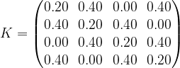If we label the points on the circle by $1, 2, \dots, N$ , then the transition matrix is given by a matrix of the form (for instance for N=4)

$K = \begin{pmatrix} 0 & \frac{1}{2} & 0 & \frac{1}{2} \\ \frac{1}{2} & 0 & \frac{1}{2} & 0 \\ 0 & \frac{1}{2} & 0 & \frac{1}{2} \\ \frac{1}{2} & 0 & \frac{1}{2} & 0 \end{pmatrix}$

More generally, we can also allow the process to stay where it is with probability 1 – p, where p is then the probability to move, which leads us to the matrix

$K = \begin{pmatrix} 1-p & \frac{p}{2} & 0 & \frac{p}{2} \\ \frac{p}{2} & 1-p & \frac{p}{2} & 0 \\ 0 & \frac{p}{2} & 1-p & \frac{p}{2} \\ \frac{p}{2} & 0 & \frac{p}{2} & 1 - p \end{pmatrix}$

Let us try to figure out whether the target distribution, given by the matrix Kⁿ for large n, somehow converges.

To see this, we do two numerical experiments. First, we can easily simulate a random walk. Suppose that we have a function draw which accepts a distribution (given by a vector p whose elements add up to one) and draws a random value according to that distribution, i.e. it returns 1 with probability p₀, 2 with probability p₁ and so on. We can then simulate a random walk on the circle as follows.

def simulate_chain(N, p, steps=100, start=5):
    chain = []
    x = start % N
    chain.append(x)
    for i in range(steps):
        x = (x  + draw([p/2.0, 1.0 - p, p / 2.0]) - 2) % N
        chain.append(x)
    return chain

Here N is the number of points on the circle, steps is the number of simulation steps that we run and start is the starting point. The function draw then returns 1 with probability p/2, 3 with probability p/2 and 2 with probability 1 – p. Thus we move with probability p/2 to the right, with probability p/2 to the left and stay were we are with probability 1 – p. If we set p = 0.8, this results in the following transition matrix.

$\begin{pmatrix} 0.20 & 0.40 & 0.00 & 0.00 & 0.00 & 0.00 & 0.00 & 0.00 & 0.00 & 0.40 \\ 0.40 & 0.20 & 0.40 & 0.00 & 0.00 & 0.00 & 0.00 & 0.00 & 0.00 & 0.00 \\ 0.00 & 0.40 & 0.20 & 0.40 & 0.00 & 0.00 & 0.00 & 0.00 & 0.00 & 0.00 \\ 0.00 & 0.00 & 0.40 & 0.20 & 0.40 & 0.00 & 0.00 & 0.00 & 0.00 & 0.00 \\ 0.00 & 0.00 & 0.00 & 0.40 & 0.20 & 0.40 & 0.00 & 0.00 & 0.00 & 0.00 \\ 0.00 & 0.00 & 0.00 & 0.00 & 0.40 & 0.20 & 0.40 & 0.00 & 0.00 & 0.00 \\ 0.00 & 0.00 & 0.00 & 0.00 & 0.00 & 0.40 & 0.20 & 0.40 & 0.00 & 0.00 \\ 0.00 & 0.00 & 0.00 & 0.00 & 0.00 & 0.00 & 0.40 & 0.20 & 0.40 & 0.00 \\ 0.00 & 0.00 & 0.00 & 0.00 & 0.00 & 0.00 & 0.00 & 0.40 & 0.20 & 0.40 \\ 0.40 & 0.00 & 0.00 & 0.00 & 0.00 & 0.00 & 0.00 & 0.00 & 0.40 & 0.20 \\ \end{pmatrix}$

We can visualize the results if we execute a large number of runs and draw histograms of the resulting positions 100, 200, 300, … steps. The result will look roughly like this (for this image, I have used p = 0.8 and N=10):

We see that after a few hundred steps, this seems to converge – actually this starts to look very much like a uniform distribution. As we already know that the distribution after n steps is given by the matrix Kⁿ, it makes sense to look at high powers of this matrix as well. To visualize this, I will use a method that I have seen in MacKays excellent book and that works as follows.

Visualizing one row of a matrix is not difficult. We can plot the entries in a two-dimensional diagram, where the x-axis corresponds to the column index and the y-axis corresponds to the value. A flat line is then a row in which all entries have the same value.

To display a full matrix, we use colors – we assign one color to each row index and plot the individual rows as just described. If we do this for the powers of the matrix K with the parameters p = 0.8 and N = 10 (and only chose some rows, for instance 1,4,7, to not run out of colors…) we obtain an image like the one below.

We can clearly see that the powers of the matrix K converge towards a matrix

$K^\infty = \lim_{n \rightarrow \infty} K^n$

where all entries in each row seem to have the same value. We have seen that the distribution after n steps assuming an initial distribution described by a row vector $\mu$ is $\mu K^n$ . Therefore the limit distribution is $\mu K^\infty$ . If we take $\mu$ to be a unit vector, we find that the rows of the matrix $K^\infty$ do actually represent the limit distribution of all chains that have started at a specific point i of the state space. Therefore the entries in the rows need to sum up to one, and thus, if they are all equal, need to be equal to 1 / N. If you calculate and print out high powers of the matrix K, you will in fact see that they approach the matrix where all entries are 0.1 (as we have chosen N = 10 in this example).

To completes our short introduction into Markov chains. We have seen that Markov chains model stochastic processes in discrete time in which the state at step t+1 depends only on the state at step t and the dependency is given by a function independent of the current time. In finite state spaces, Markov chains are described by a transition matrix K. The i-th row of the matrix Kⁿ is the distribution of chains starting at point i after n steps. Consequently, converge properties of the Markov chains can be related to converge of high powers Kⁿ and the apparatus of linear algebra can be applied.

In the next post, we will learn more about convergence – how it can be made precise, and how we can tell whether a given Markov chain converges. This will then allow us to construct Markov chains that converge towards a given target distribution and use them for sampling.

Monte Carlo methods and Markov chains – an introduction

In our short series on machine learning, we have already applied sampling methods several times. We have used and implemented Gibbs sampling, and so far we have simply accepted that the approach works. Time to look at this in a bit more detail in order to understand why it works and what the limitations of the algorithm are.

Regardless of whether you want to simulate ferromagnetic behavior in an Ising model, run a Hopfield network or train a Boltzmann machine, the fundamental problem that we have to solve is always the same. We are given a probability distribution P living on some state space X, and we are trying to create a sample, i.e. a set of points in the state space such that the probability for a point x to appear in this sample is equal to the probability P(x) given by the probability distribution.

The naive approach to this is simple: visit every point x in the state space and include that point with probability P(x). However, it is clear that with a large state space, this approach is not computationally feasible. In the example of a Boltzmann machine trained on handwritten digits with 28 x 28 pixels, our state space has 2⁷⁸⁴ elements, and there is no way we can visit them all one by one. Instead, we would need something like a randomized walk through the state space. We could start with same randomly chosen state X₀, then – using a randomized transition rule – move on to a point X₁ and so forth. Intuitively, we want to select our transition rule in such a way that the state space elements X_i selected in this way form a sample, i.e. such that our chain of state space locations visits regions with large values for P(x) more often than regions with low values of P(x). Thus we would systematically ignore regions of the state space with low probability which would greatly reduce the number of states that we have to visit to obtain a valid sample.

So, from a mathematical point of view, we consider a sequence of random variables X_i such that X_i+1 is related to X_i by some randomized transition rule. We also assume that this rule does not depend on the index i which is usually called the time. Thus we have a sequence of random variables X_i which is not independent, but almost independent – X_i+1 depends only on X_i and in way that itself does not vary with i. This is called a Markov chain (more precisely, a time homogeneous Markov chain).

Let us consider an example to illustrate the idea. As our state space, we choose the space or real numbers. We fix a starting value, say X₀=0, and we obtain the next value by adding a number that we draw from a standard normal distribution. Thus, mathematically, we assume that W_n are identically distributed and independent random variables, all distributed according to the standard normal distribution, and set

$X_{n+1} = X_n + W_n$

This is a Markov chain: the value X_n+1 depends only on X_n, not on any earlier elements of the chain. The transition rule is randomized, but itself does not depend on the time step n – all W_n have the same distribution. Let us implement this in Python to see how it works (the full notebook can be downloaded here).

Sorry, something went wrong. Reload?

Sorry, we cannot display this file.

Sorry, this file is invalid so it cannot be displayed.

view raw GaussianRandomWalk1.ipynb hosted with ❤ by GitHub

Here we have created and displayed three different random walks. All of them start at the same point (zero), and all of them follow the same transformation rule, but as the transformation rule is stochastic in nature, they all develop differently.

Now let us try to turn the view on this upside down. This time, we execute a larger number – 1000 – of random walks with 5000 steps each. But instead of plotting the sequence of points X_i for every walk, we display the distribution of the last point of each walk, i.e. we plot the distribution of the random variable X₄₉₉₉.

Sorry, something went wrong. Reload?

Sorry, we cannot display this file.

Sorry, this file is invalid so it cannot be displayed.

view raw GaussianRandomWalk2.ipynb hosted with ❤ by GitHub

This does in fact look more familiar. We see that most walks end up being close to zero at the end – steps in the positive direction and steps in the negative direction cancel each other. Only very few walks end up at an extreme position close to plus or minus 200 – this is not surprising as well, to arrive at an extreme point, we would need to draw 5000 times in a row an extreme value from the random normal distribution, which is a rather unlikely chain of events.

In this case, the distribution does actually not converge if we increase the number of steps – you can try this out and play with different values, i.e. replace 5000 by 50000 (this will run some time) and look at the distribution of X₄₉₉₉₉ – you will see that this is now spread out to roughly plus / minus 750 (in fact, the distribution is obtained as a multiple convolution of the standard normal distribution with itself and thus is again a normal distribution).

Even though the distribution does not converge, we have been able to sample from a specific distribution – in this case the distribution after 5000 steps – using only the ability to sample from a different distribution – in this case the random normal distribution. Obviously, in this special case, the result is trivial, but the principle that we have found looks interesting. Can we generalize this approach to obtain sampling methods for target distributions that are otherwise intractable?

Now this is exactly the idea behind the sampling approach that is commonly known as Markov chain Monte Carlo (MCMC) and which has become very popular, with applications to complex simulations in theoretical physics, to machine learning and even asset pricing and value-at-risk calculations.

So let us summarize how the MCMC approach works. Given a target distribution P(x), we first construct a Markov chain that converges to that target distribution. Once we have that, we can simulate a large number of runs and use the resulting points as our sample (in fact, in many cases we can also do with one run only, as we will see later). Thus in order to utilize Markov chains for sampling, we would need to understand under what conditions a Markov chain converges and if it converges, how we can relate the target distribution to the transformation rule. We will look into these points in more detail in future posts in this series.

Training restricted Boltzmann machines with persistent contrastive divergence

In the last post, we have looked at the contrastive divergence algorithm to train a restricted Boltzmann machine. Even though this algorithm continues to be very popular, it is by far not the only available algorithm. In this post, we will look at a different algorithm known as persistent contrastive divergence and apply it to the BAS data set and eventually to the MNIST data set.

Recall that one of the ideas of contrastive divergence is to use a pattern from the sample set as a starting point for a Gibbs sampler to calculate the contribution of the negative phase to the weight update. The idea behind persistent contrastive divergence (PCD), proposed first in [1], is slightly different. Instead of running a (very) short Gibbs sampler once for every iteration, the algorithm uses the final state of the previous Gibbs sampler as the initial start for the next iteration. Thus, in every iteration, we take the result from the previous iteration, run one Gibbs sampling step and save the result as starting point for the next iteration.

This amounts to running one long chain of states that are related by Gibbs sampling steps. Of course this is not exactly one longs Gibbs sampler, as the weights and therefore the probability distribution changes with each step. However, the idea is that when the learning rate is small, the weight change during two subsequent iterations is neglegible, and we effectively create one long Gibbs sampler which provides a good approximation to the actual distribution.

In practice, one often uses several chains that are run in parallel. Such a chain is sometimes called a negative particle. It is recommended in [1] to chose the number of particles to be equal to the batch size. In an implementation in Python, we can store the state of the negative particles in a matrix N where each row corresponds to one particle.

The idea to form one long Markov chain obviously works best if the learning rate is very small. On the other hand, this slows down the convergence of the gradient descent algorithm. In order to solve this, it is common to reduce the learning rate over time, for instance linearly with the number of iterations.

A second additional improvement that is usually implemented is a weight decay. Essentially, a weight decay is an additional penalty that is applied to avoid that the weights grow too large which would slow down the sampling procedure.

Let us now see how the PCD algorithm can be coded in Python. We will again store the model parameters and the state in a Python class. In the __init__ method of that class, we initialize the weights and the bias vectors and also set the particles to some randomly chosen initial value.

class PCDRBM (Base.BaseRBM):

    def __init__(self, visible = 8, hidden = 3, particles = 10, beta=2.0):
        self.visible= visible
        self.hidden = hidden
        self.beta = beta
        self.particles = particles
        #
        # Initialize weights with a random normal distribution
        #
        self.W = np.random.normal(loc=0.0, scale=0.01, size=(visible, hidden))
        #
        # set bias to zero
        #
        self.b = np.zeros(dtype=float, shape=(1, visible))
        self.c = np.zeros(dtype=float, shape=(1, hidden))
        #
        # Initialize the particles
        #
        self.N = np.random.randint(low=0, high=2, size=(particles,self.visible))
        self.global_step = 0

Assuming that we have a method runGibbsStep that runs one Gibbs sampling step with the given weight starting at some initial state, one iteration of the PCD algorithm now looks as follows.

#
# Update step size - we do this linearly over time
#
step = initial_step_size * (1.0 -(1.0*self.global_step)/(1.0*iterations*epochs))
#
# First we compute the negative phase. We run the
# Gibbs sampler for one step, starting at the previous state
# of the particles self.N
#
self.N, _ = self.runGibbsStep(self.N, size=self.particles)
#
# and use this to calculate the negative phase
#
Eb = expit(self.beta*(np.matmul(self.N, self.W) + self.c))
neg = np.tensordot(self.N, Eb, axes=((0),(0)))
#
# Now we compute the positive phase. We need the
# expectation values of the hidden units
#
E = expit(self.beta*(np.matmul(V, self.W) + self.c))
pos = np.tensordot(V, E, axes=((0),(0)))
#
# Now update weights
#
dW = step*self.beta*(pos -neg) / float(batch_size) - step*weight_decay*self.W / float(batch_size)
self.W += dW
self.b += step*self.beta*np.sum(V - self.N, 0) / float(batch_size)
self.c += step*self.beta*np.sum(E - Eb, 0) / float(batch_size)
self.global_step +=1

As always, the full source code is available from my machine learning GitHub repository. I have enhanced the code in RBM.py so that it accepts a command line parameter --algorithm that lets you choose between ordinary contrastive divergence and the PCD algorithm.

Let us now run a few trials. First, we will again use the BAS data set. You can download and run the code from the GitHub repository as follows.

$ git clone http://www.github.com/christianb93/MachineLearning.git
$ cd MachineLearning
$ python RBM.py --algorithm=PCD --run_reconstructions=1 --show_metrics=1

When the script completes, you should again see the two images. The first image displays how the reconstruction errors and weight changes behave during the training.

We see that the reconstruction error (the diagram on the right) decreases slower than it did for the ordinary contrastive divergence algorithm. On the left hand side, where the change of the weights is displayed, we can clearly see the impact of the linearly decreasing step size. The second picture shows again the result of a reconstruction attempt of slightly distorted patterns.

Let us now try out a different application of restricted Boltzmann machines – sampling. After a successful training phase, the model distribution given by the weights should be close to the empirical distribution of the training data. Thus, if we sample from the model distribution, using for instance Gibbs sampling, we should be able to obtain patterns. that somehow resemble the training data.

We will use this to generate handwritten digits based on the well known MNIST data set, more precisely the copy available at mldata.org. To download and read the data set, we use the method fetch_mldata provided by the scikit learn library. We will then train our network for 40.000 epochs using 60 images out of this data set and 128 hidden units and subsequently run 200.000 Gibbs sampling steps starting from a random pattern.

$ python RBM.py --algorithm=PCD --data=MNIST --N=28 --epochs=40000 --pattern=60 --hidden=128 --run_samples=1 --sample=200000 --save=1

Note that when you run this for the first time, the MNIST data set will be downloaded and stored in a folder in your home directory, so this might take some time (the file has a bit less than 60 MBytes).

The results are already very encouraging. Most patterns resemble a digit closely, only the image at the top left corner did obviously not converge properly. However, we still see a strong bias – only very few of the 9 digits that the data set contains appear. So we probably need to fine tune the parameters like number of hidden units, learning rate, weight decay or the number of epochs to obtain better results.

Unfortunately, when you start to play around to optimize this further, you will see that the run time of the algorithm has reached a point where quick iterations to try out different parameters become virtually impossible. I have been running this on my PC that has an Intel Core i7 CPU, and Python was able to distribute this nicely across all four physical cores, taking them to 100% utilization, but still the script was already running for 7 minutes. If we want to increase the number of iterations or the number of hidden units to be able to learn more pattern, the run time can easily go up to almost 30 minutes.

Of course professional training of neuronal networks is nowadays no longer been done on a CPU. Instead, modern frameworks use the power of graphical processing units (GPUs) that are optimized for exactly the type of work that we need – highly parallel processing of floating point matrices. Therefore, I will show you in the next post in this series how you can use the TensorFlow framework to move the workload to a GPU.

1. T. Tieleman, Training restricted Boltzmann machines using approximations to the likelihood gradient, International Conference on Machine Learning (ICML), 2008
2. A. Fischer, C. Igel, Training restricted Boltzmann machines: an introduction, Pattern Recognition Vol. 47 (2014), pp 25–39