Machine learning – Page 5

The Ising model and Gibbs sampling

In the last post in the series on AI and machine learning, I have described the Boltzmann distribution which is a statistical distribution for the states of a system at constant temperature. We will now look at one of the most important applications of this distribution to an actual model, the Ising model.

This model was proposed by W. Lenz and first analysed in detail by his student E. Ising in his dissertation (of which [1] is a summary) to explain ferromagnetic behavior. In Isings model, a solid, like a piece of iron, is composed of a large number N of individual particles, each of them at a fixed location. A particle acts as a magnetic dipole that can be oriented in two different ways, corresponding to the different orientations of its spin. Ignoring the spatial structure for the time being, we can thus describe the state of the model as a point in the state space

${\mathcal S} = \{ -1, 1\}^N$

We denote the elements of the state space by s and the i-th spin by $s_i \in \{-1,1\}$ where a value of +1 is interpreted as “spin up” and a value of -1 as “spin down”.

Now, in general, a magnetic dipole which is exposed to a magnetic field B and has a magnetic dipole moment m will have a potential energy

$E = - m \cdot B$

which is the scalar product of m and B, i.e. the state of minimum energy is the one where the dipole is oriented along the magnetic field. In a solid, there are two sources for the magnetic field that act on each particle – there might be an external magnetic field H and there might be an interaction with the other magnetic dipoles in the model. We therefore model the total energy of a state s as

$E(s) = - \frac{1}{2} \sum_{i,j} J_{ij} s_i s_j - \sum_j h_j s_j$

where $J_{ii} = 0$ (i.e. we exclude self-interactions).

Here the coefficient $h_j$ represents the external field acting on the particle at position j. The matrix J represents the interactions between the particles. In Isings original model, only nearby particles interact. In two dimensions, for instance, we think of the particles as being located on a grid and each particle has four neighbors: the particles immediately above and below it and the particles on the left and on the right. We can define a model which has a boundary or we can think of the grid as being toroidal, i.e. wrapping around.

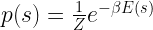
We now consider the system as being in contact with a heat bath at a certain temperature T, i.e. the system can exchange internal energy with a thermal reservoir, leading to fluctuations in the orientations of the particles. This appears to be a reasonable model, we could, for instance, consider a comparatively small part of a solid and take the surrounding, much larger solid as the heat bath. The probability for the system to be in a state s is therefore given by the Boltzmann distribution:

$p(s) = \frac{1}{Z} e^{-\beta E(s)}$

The macroscopic quantities that are of primary interest are of course the average energy, but also the magnetization

$M(s) = \frac{1}{N} \sum_i s_i$

and its average value. At high temperatures and for H = 0, we expect that roughly half of the spins should be oriented in either direction, so the average magnetization should be zero. If we add an external field, then of course most of the dipoles will be aligned in the direction of this field, so the magnetization will be close to one or minus one. This fact – magnetization of a solid in the presence of an external magnetic field – is called paramagnetism. It turns out that for some materials, a non-zero magnetization can occur even if the external field is zero, as long as the temperature is below a certain value called the critical temperature – this behavior is known as ferromagnetism. Explaining this macroscopic behavior by a statistical model was the original intention of Isings work.

Now how do we actually evaluate our model? Our aim is to determine – for instance – the average magnetization at a given temperature. To do this naively, we would have to calculate the probabilities for all possible states s. Unfortunately, the number of states grows exponentially with the number N of particles. Suppose we wanted to use a toy model with only 40 x 40 spins – this is very small compared to the number of particles in an average macroscopic solid. As N = 1600 in this case, we would have $2^{1600}$ different states, which is roughly $10^{482}$ . Comparing this to the estimated age of the universe in seconds ( $4 \cdot 10^{17}$ , see for instance this page), it is obvious that this is not a good idea.

However, we can try to approximate the average magnetization by using a sufficiently large sample. Thus we try to find a set of states $s_i$ which is large, but doable – maybe a few million – and hope, based on the law of large numbers, that the sample average, i.e. the sum $\sum_i M(s_i)$ , will provide a good approximation for the real value. This approach is sometimes called Monte Carlo integration and the workhorse of computational statistical mechanics.

How, then, do you create that sample? The answer is easy to write down, but difficult to motivate without the necessary background on Markov chains. Thus I will simply state the algorithm which is called Gibbs sampling and leave the theoretical background to another post (for the mathematically inclined reader, it is worth mentioning that the sample produced by the Gibbs sampler is not independent, but the law of large number still holds).

Before we can phrase the algorithm, we need another preparational step – we need to calculate a conditional probability. Suppose that the system is in a state s and we have chosen an arbitrary coordinate i. We can then ignore the actual state of the spin $s_i$ and ask for the conditional probability that this spin points upwards given all other spins. A not too difficult calculation (which is carried out in detail for instance in my notes) shows that this conditional probability is given by

$P(s_i = 1 | \{ s_j\}_{j \neq i}) = \sigma(2 \beta ( \langle J_i, s \rangle + h_i))$

Here $J_i$ denotes the i-th row of the matrix J and the brackets denote the ordinary scalar product. With this expression, a single Gibbs sampling step now proceeds as follows, given a state s.

Randomly pick a coordinate i
Calculate the conditional probability $P = P(s_i = 1 | \{ s_j\}_{j \neq i})$ using the formula above
Draw a real number U between 0 and 1 from the uniform distribution
If U is at most equal to P, set the spin at position i to +1, otherwise set it to -1

The algorithm then starts with a randomly chosen state and subsequently applies a large number of Gibbs sampling steps. After some time, called the burn-in time, the states after each step then form the sample we are looking for.

After all that theory, let us now turn to the practical implementation. We will restrict ourselves to the original model, i.e. $J_{ij} = 1$ if particles i and j are neighbors and zero otherwise, and also set the magnetic field to zero. The Gibbs sampling algorithm as outlined above is straightforward to implement in Python. You can get my code from GitHub as follows.

$ git clone https://github.com/christianb93/MachineLearning.git

In the newly created directory MachineLearning, you should then see a file Ising.py. Run this as follows.

$ python IsingModel.py

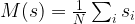
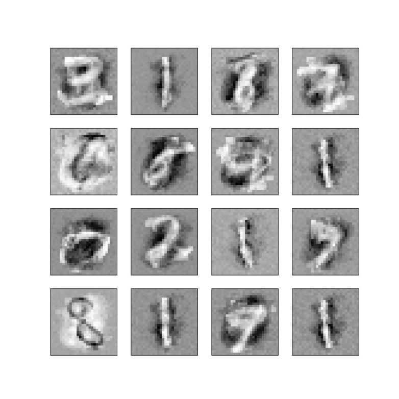
This will create a new temporary directory with a name that is unique and specifies the run (on Linux / Unix systems, you will find the newly created directory in /tmp/. In this subdirectory, you will find three files. A file with extension .txt summarizes the parameters of the run. The file that ends with IsingPartI.png displays the simulation results. An example is

Each of the little images represents one final state for a given temperature. In this example, a grid of 40 x 40 spins was calculated. The temperature was slowly decreased from 6.0 down to 0.2 in steps of 0.2. For each temperature, 4 million simulation steps were done, then the resulting grid was captured. The top row represents, from the left to the right, the temperatures 6.0, 5.8, 5.6, 5.4 and 5.2. Here we see the expected behaviour – patterns with roughly half of the particles in a spin-up position and half of the particles in a spin-down orientation.

In the bottom row of the diagram, that corresponds to the temperatures 1.0, 0.8, 0.6, 0.4 and 0.2, we also see the expected behavior for very low temperatures – all spins are oriented in the same direction. However, starting at temperatures 1.8, we see that large scale patterns start to emerge. especially for the temperatures 2.2 and 2.4 (rightmost pictures in the fourth row from the top). For these temperatures, entire connected regions display the same orientation of the spins and thus a non-zero mean magnetization. As the temperature rises, these patterns dissolve again.

This behaviour is typical for a so-called critical point and is what Ising was searching for. Ironically, Ising, who of course did not have the computational devices to run a simulation, concluded in his paper wrongly that this would not happen. Critical points are of great interest not only in statistical mechanics, but also in quantum field theory – we will not be able to explore this connection further, but it demonstrates how important the Ising model has become as a playground to bring together various branches from physics, computer science and mathematics.

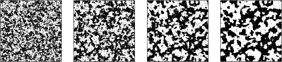
The program has lots of parameters to play with – with the default values, for instance, it calculates comparatively small grids with 20 x 20 spins, so that a small number of iterations is sufficient, for larger grids you will need several million iterations. I recommend to play with this a bit to get a feeling for what happens. The image at the top of this article, for instance, was generated with the following command line:

$ python IsingModel.py --show=1 --N=160000 --rows=400 --cols=400 --steps=100000 --Tmax=2.4 --Tmin=1.7

and ran for roughly 13 minutes on my PC.

It is worth mentioning that neither the Gibbs sampling algorithm nor the chosen implementation are optimized. In fact, there are other algorithms like the exact sampling algorithm (see for instance [2]) that are providing much better results, and also the implementation could be improved greatly, for instance by using a Metropolis-Hastings checkerboard algorithm to allow for high parallelization and GPU computing (see for instance [3]). However, as understanding Gibbs sampling is vital for understanding Boltzmann machines, I have chosen to use a down-to-earth Gibbs sampling approach for this post – after all, its main purpose is not to gain new physical insights from simulation results but to get acquainted with Gibbs sampling as a standard sampling method, and, as always, to have some fun.

If you would like to learn more on the Ising model, please have a look at my notes that provide more details, show how to compute the conditional probability used for the Gibbs sampling and also cover the one-dimensional Ising model.

In the meantime, you might want to take a look at the beautiful article of J. Harder on WordPress who has some more sample pictures and a very interesting application of convolutional neuronal networks that he trained to be able to determine the temperatue at which the simulation was run from the visual representation of the simulation result.

References

1. E. Ising, Beitrag zur Theorie des Ferromagnetismus,
Zeitschrift f. Physik, Vol. 31, No.1 (1924), 253-258
2. D. MacKay, Information Theory, Inference and Learning Algorithms, Cambridge University Press, Cambridge 2003
3. M. Weigel, Simulating spin models on GPU, Computer Physics Communication 182 (2011), 1833-1836

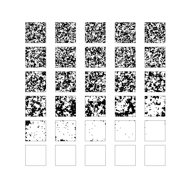
The Boltzmann distribution

Boltzmann machines essentially learn statistical distributions. During the training phase, we present them a data set called the sample data that follows some statistical distribution. As the weights of the model are adjusted as part of the learning algorithm, the statistical model represented by the Boltzmann machine changes, and the learning phase is successful if the model gets as closely to the training data as possible.

The distribution that is learned by a Boltzmann machine is called a Boltzmann distribution (obviously, this is where the name comes from…) and is of great importance in statistical physics. In this post, we will try to understand how this distribution arises naturally from a few basic assumptions in statistical mechanics.

The first thing that we will need is a state space. Essentially, a state space is a (probability) space whose points are in one-to-one correspondence with the physical states of the system that we want to describe. To illustrate this, suppose you are given a system of identical particles. These particles can move freely in a certain are of space. The location of each individual particle can be described by its location in space, thus by three real numbers, and its velocity is described by three additional real numbers, one for each spatial component of the velocity. Thus as a state space for a single particle, we could choose a six-dimensional euclidian space. For a system of N particles, we would therefore need a state space of dimension 6N.

But a state space does not need to be somehow related to a position in some physical space. As another example, consider a solid, modeled as N particles with fixed locations in space. Let us also assume that each of these particles has a spin, and that this spin can either point upwards or downwards. We could then describe the spin of an individual particle by +1 (spin up) or -1 (spin down), and therefore our state space for N particles would be

$\Omega = \{-1, +1\}^N$

For every point s in the state space, i.e. for every possible state of the system, we assume that we can define an energy E(s), so that the energy defines a function E on the state space. One of the fundamental questions of statistical physics is now:

Given a state space and an energy function E on that space, derive, for each state s, the probability that the system is in the state s

What exactly do we mean by the probability to be in a specific state? We assume that we could theoretically construct a very large number of identical systems that are isolated against each other and independent. All these systems evolve according to the same rules. At any point in time, we can then pick a certain state and determine the fraction of systems that are in this state. This number is the probability to be in that state. The set of all these systems is called a statistical ensemble. The assignment of a probability to each state then defines a probability distribution on the state space. To avoid some technicalities, we will restrict ourselves to the case that the state space is finite, but of course more general cases can be considered as well.

As it stands, the question phrased above is impossible to answer – we need some additional assumptions on the system to be able to write down the probability distribution. We could, for instance, assume that the number of particles and the energy are fixed. A bit less restrictive is the assumption that the energy can vary, but that the temperature of the system (and the number of particles as well as the volume) is fixed – this is then called a canonical ensemble. Let us denote the temperate by T and assume now that it is constant.

We could describe a system for which these assumptions hold as being in contact with a second, very large system which is able to supply (or absorb) a virtually infinite amount of heat – this system is called a heat bath or thermal reservoir. The composite system that consists of our system of interest and the heat bath is assumed to be fully isolated. Thus its energy and the number of particles is constant. Our primary system can exchange heat with the heat bath and therefore its energy can change, while its temperate will stay constant and equal to the temperature of the heat bath.

Let us denote the energy of the overall system by $U_{tot}$ , its entropy by $S_{tot}$ , the energy of the heat bath by $U_R$ and the entropy of the heat bath by $S_R$ (if energy and entropy are new concepts for you, I recommend my short introduction to thermodynamics which summarizes the most important fundamentals of thermodynamics on roughly 40 pages and also contains more details on statistical ensembles and the Boltzmann distribution).

Now it turns out that making only these very general assumptions (in contact with heat bath, constant temperature) plus one additional assumption, we can already derive a formula for the probability distribution on the state space – even without knowing anything else on the state space! Let me sketch the argument to get a feeling for it, more details can be found in the document mentioned above.

Let us assume that we are given some state s of our primary system with energy E(s). We can combine this state with a state of the heat bath to an allowed state of the composite system if the energies of both states add up to the total energy $U_{tot}$ , i.e. with any state of the heat bath which has energy $U_{tot} - E$ . Let us denote the number of states of the heat bath with that energy by

$W_R(U_{tot} - E)$

and let $W_{tot}$ denote the number of states of the composite system with energy $U_{tot}$ . The major additional assumption that we now make is that for the composite system, all states with energy $U_{tot}$ are equally likely – this is known as the principle of indifference.

Let us take a moment to reflect on this. The principle of indifference (sometimes called the principle of insufficient reason) states (translated into our case) that if the states of the system cannot be distinguished by any of the available observable quantities (in this case the energy which is equal to $U_{tot}$ for all states of the composite system), all these states should be assigned equal probabilities. This appears somehow reasonable, if one state was more likely than any other state, this state would somehow be distinguished but could not be told apart by any of the measurable quantities. Of course, that something is not measurable does not mean that it does not exist – there could even be a quantity that is theoretically observable and distinguishes certain states, but is simply not on our radar. So this principle has to be applied with care, but it turns out that the resulting distribution gives a surprisingly good description of what we can measure in a large number of applications, so this assumption is somehow justified by its success (see also {1] chapter 15 and 21 for a short discussion and justification).

What does the principle of indifference imply for our primary system? The number of states of the composite system for which our primary system is in state s is exactly $W_R(U_{tot} - E)$ , because every such state combines with s to an admissible state of the composite system. If all these states are equally likely, the probability for s is therefore just the fraction of these states among all possible states of the composite system, i.e.

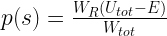
$p(s) = \frac{W_R(U_{tot} - E)}{W_{tot}}$

The beauty of this equation is that we can express both, the numerator and the denominator, by the entropy. And this is where finally the Austrian physicist Ludwig Boltzmann comes into play. Boltzmann identified the entropy of a system with the logarithm of the number of states available to the system – that is the famous relation that is expressed as

$S = k \ln W$

on his tomb stone. Here W is the number of states available to the system, and k is the Boltzmann constant.

Let us now use this expression for both numerator and denominator. We start with the denominator. If the system has reached thermal equilibrium, the primary system will have a certain energy U which is related to the total energy and the energy of the reservoir by

$U_{tot} = U + U_R$

Using the additivity of the entropy, we can therefore write

$W_{tot} = \exp \frac{1}{k} \left[ S(U) + S_R(U_{tot} - U) \right]$

Observe that we assume the number of particles and the volume of both the reservoir and the composite system to be constant, so that the entropy does really only depend on the volume (or at least we assume that the dependency on the volume is negligible). For the numerator, we need a different approach. Let us try a Taylor expansion around the energy $U_{tot} - U = U_R$ . The first derivative of the entropy with respect to the energy is – by definition – the inverse of the temperature:

$\frac{\partial S_R}{\partial U_R} = \frac{1}{T}$

The second derivative turns out to be related to the heat capacity $C_R$ of the reservoir. In fact, we have

$\frac{\partial}{\partial U_R} \frac{1}{T} = - \frac{1}{T^2 C_R}$

Now a heat bath is characterised by the property that we can add a virtually infinite amount of heat without raising the temperature. Thus the heat capacity is infinite, and the second derivative is (virtually) zero. Therefore our Taylor expansion is

$S_R(U_{tot} - E(s)) = S_R(U_{tot} - U) + \frac{1}{T} (U - E(s))$

Putting all this together, a few terms cancel out, and we find that

$p(s) = \exp \frac{1}{kT} \left[ (U - TS(U)) - E(s) \right]$

Now the energy U is the average, i.e. the macroscopically observable, energy of the primary system. Therefore $U - TS$ is the Helmholtz energy $F$ . If we also introduce the usual notation $\beta$ for the inverse of $kT$ , we finally find that

$p(s) = e^{\beta F} e^{- \beta E(s)}$

This is usually written down a bit differently. To obtain this form, let us sum this over all possible states. As U and therefore F are averages and do not depend on the actual state, but all probabilities have to add up to one, we find that

$1 = e^{\beta F} \sum_s e^{- \beta E(s)}$

The last sum is called the partition function and usually denoted by Z. Therefore we obtain

$p(s) = \frac{1}{Z} e^{- \beta E(s)}$

which is the Boltzmann distribution as it usually appears in textbooks. So we have found a structurally simple expression for the probability distribution, starting with a rather general set of assumptions.

Note that this equation tells us that the state with the lowest energy will have the highest probability. Thus the system will prefer states with low energies, and – due to the exponential – states with a significantly higher energy tend to be very unlikely.

Due to the very mild assumptions, the Boltzmann distribution applies to a large range of problems – it can be used to derive the laws for an ideal gas, for systems of spins in a solid or for a black body. However, the formula is only simple at the first glance – the real complexity is hidden in the partition function. With a few short calculations, one can for instance show that the entropy can be derived from the partition function as

$S = k \frac{\partial}{\partial T} T \ln Z$

Thus if we known the partition function as a function of the macroscopic variables, we know all the classical thermodynamical quantities like entropy, temperature and Helmholtz energy. In many cases, however, the partition function is not known, and we have to devise techniques to derive physically interesting results without a tractable expression for the partition function.

That was it for today. This blog was a bit theoretical, so next time we will apply this to a concrete model which is accessible for numerical simulations, namely the Ising model. Until then, you might want to go through my notes which contain some details on the Boltzmann distribution as well as examples and applications.

References

1. H.B. Callen, Thermodynamics and an introduction to thermostatistics, 2nd edition, John Wiley 1985
2. D.V. Schroeder, An introduction to thermal physics, Addison Wesley 2000

Boltzmann machines, spin, Markov chains and all that

The image above displays a set of handwritten digits on the left. They look a bit like being sketched on paper by someone in a hurry and then scanned and digitalized, not very accurate but still mostly readable – but they are artificial, produced by a neuronal network, more precisely a so called restricted Boltzmann machine.

On the right hand side, you see the (core part of) the code that has been used to produce this image. These are about forty lines of code, and there is some code around it which is not shown, but stripping off all the comments and boilerplate code, we could probably fit the algorithm into less than fifty lines of code.

I found this contrast always fascinating. Creating something that resembles handwritten digits sounds incredibly complex, but can be done with an algorithm that can be quenched into a comparatively short program – how does that work? So I started to dig deeper, trying to understand neuronal networks in general and in particular Boltzmann machines – the mathematical foundations, the algorithm and the implementation.

Boltzmann machines are a rather special class of neuronal networks that have a reputation of being hard to train, but are important from a theoretical point of view, being closely related to seemingly remote fields like thermodynamics, statistical mechanics and stochastical processes. That makes them interesting, but also hard to understand. I embarked on that journey a couple of months ago, and I thought it would be nice to create a series of blog posts on this. My current thinking is to have one or two posts on each of the following topics over the next couple of weeks.

Overview – what are Boltzmann machines (this post)
Background from statistical mechanics and the Boltzmann distribution
The Ising model and Gibbs sampling
Hopfield networks: theory
Hopfield networks: practice
From Hopfield networks to Boltzmann machines
Restricted Boltzmann machines
Contrastive divergence and PCD
Implementation with TensorFlow
Basics of Markov chains
Finite Markov chains and recurrent Markov chains
The Metropolis Hasting algorithm

This is a lot of content, and please do not expect to see one post every other day. But maybe I should just start and we will see how it goes….

So let me try to roughly sketch what a Boltzmann machine is. First, it is a neuronal network. As such it is composed of units that can be compared to the neurons in the nervous system. Similar to a neuron, each unit has an input and an output. The output of a neuron can serve as input for another neuron. In general, every neuron receives inputs from many other neurons and delivers outputs to many other neurons.

The diagram above shows a very simple neuronal network. It consists of four neurons. The three of them on the left serve as input to the network. Think of them as the equivalent of cells in – say – your visual cortex that are activated by some external stimulus. The cell on the right is the output of the network. Its activation is computed based on the outputs of the neurons on the left and some parameters of the network called the weights which model the strength of the connection between the neurons and which we denote by $w_i, i = 0, 1, 2$ , as follows.

$o = \sigma(w_0 x_0 + w_1 x_1 + w_2 x_2) = \sigma(w^T X)$

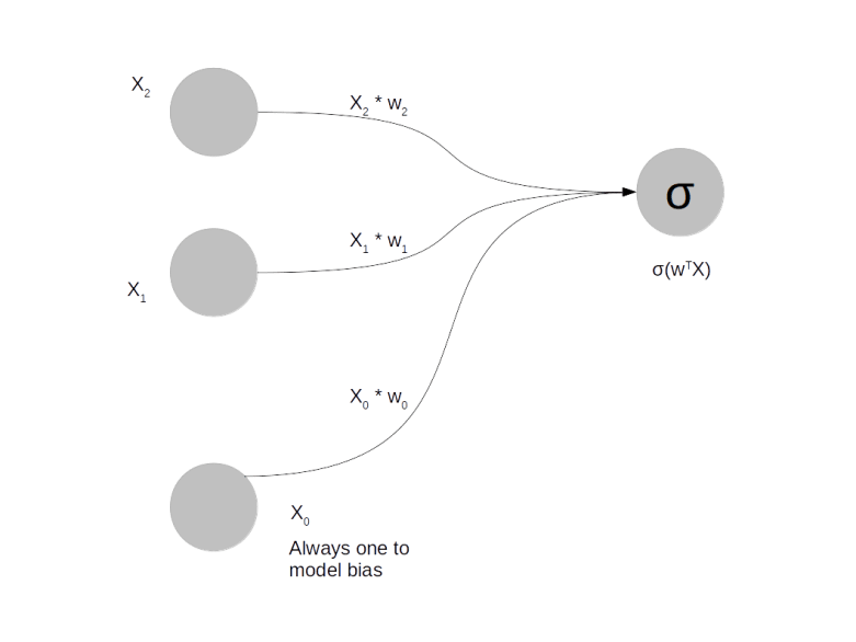
Here $\sigma$ is a function called the activation function and $X$ is the vector that is formed by $x_0, x_1$ and $x_2$ . There are a few standard choices for the activation function, a common one being the sigmoid function.

How is such a network applied? Let us look at this for a problem which is the “Hello World” of machine learning – recognition of handwritten digits. In that problem, you start with a collection of digitized images of handwritten digits, like those that are known as the MNIST database. These images have 28×28 = 784 pixels. We want to design a neuronal network that can classify these images. Such a network should consequently have 784 input units and 10 output units (bear with me that I did not produce a picture of that network, even though it would probably be fun to do this with Neo4J). We present an image to the network by setting the value of the input unit i to the intensity of pixel i. Our aim is to adjust the weights in such a way that if the image represents digit n, only output n is significantly different from zero. This will allow us to classify unknown images – we simply present the image to the network and then see which output is activated.

But how do we find the correct values for the weights? We need weights that connect each of the ten output units to each of the 784 input units, i.e. we have 7840 weights. Thus we are looking for a point in a 7840 dimensional vector space – not easy. Here the process of training comes into play. We take our set of sample images and present them to the network, with initially randomly chosen weights. The output will then not be what we want, but differ from the target output by an error. That error can be expressed as a function of the weights. The task is then to find a minimum of the error function, and there are ways to do this, most notably the procedure which is known as gradient descent.

As the name suggests, we need the gradient of the error function for that purpose. Fortunately, for the type of neuronal network that we have sketched so far, the gradient can be computed fairly easily – in fact the activation function is chosen on purpose to make dealing with the derivatives easy. We end up with a comparatively simple training algorithm for this type of network and maybe I will show how a simple implementation in Python in a later post – but for now let us move on to Boltzmann machines.

Boltzmann machines or more precisely restricted Boltzmann machines (RBMs) are also composed of units and weights, but work a bit differently. There are inputs, which are usually called visible units. But there are no classical outputs. Instead, there is a layer of units that is connected to the visible units and is called hidden units, as shown in the following picture.

In the example of handwritten digits again, you would again have 784 visible units. However, the hidden units would not obviously correlate with the digit represented by the input. Instead, you would have a more or less arbitrary number of hidden units, say 300.

During training, you present the network one image, again by setting the values of the visible units (the input) to the pixel intensities. You then compute the value of the hidden units – but you do not do this deterministically, but bring in some random element. Roughly speaking, if the combined input to a hidden unit is p, you set the value of the unit to one with probability p. Then this process is repeated, this time starting from the hidden units. This gives you certain values for the visible units. You then compare this value to the original value and try to adjust the weights such that you get as closely as possible to the original input (this is not exactly true and a not very precise description of one of the possible learning algorithms called contrastive divergence, but we will get more precise later on).

If you succeed, you will be able to reconstruct the value of the visible units from the values of the hidden units. But there are less hidden units, so that the network has apparently learned a condensed representation of the input that still captures the essence of the input. In the case of digits, you can visualize the state of the network after training and obtain something like

These are visualizations of the weights connected to some of the hidden units of a Bolzmann machine after the training phase. We can see that some of the units have appearantly “learned” some characteristic features of the digits, like the vertical stroke that appears in the digits one and seven. These features can be used for several purposes.

First, we can use the features as input for other neuronal networks. We now have only 300 inputs instead of originally 784, and that might simplify the problem a bit and make the process of training the next network easier.

Or, we could start with some random values for the hidden units and calculate the resulting values of the visible units to create sample images – and in fact this is basically what I have done to produce the samples at the top of this post (using an algorithm called PCD, but we will get to this).

Note that Boltzmann machines differ significantly from the type of neural network that we have considered earlier. One major difference is that to train a Boltzmann machine, you do not need to know the digit that the image represents. At no point have we used the information that the images in our database represent ten different digits – that information was not used in the design of the network nor during the training. This approach to machine learning is called unsupervised learning and is obviously very versatile – you do not have to tell the machine what the structure of the data is, it will detect the features independently.

Second, a Boltzmann machine can not only classify images, but can also create images that resemble a given set of input data. That can be used to reconstruct partially available images or to create new images from scratch – networks with this ability are called generative networks.

The price we have to pay for this is that Boltzmann machines are hard to train. The point is that we can still define some sort of error function, but we cannot easily calculate its gradient – there is no straightforward analytic expression for it that could be evaluated within a reasonable amount of time (if you know statistical physics a bit, that might remind you of the partition function, and that is more than pure coincidence, as I will show you in a later post). So we need to approximate the gradient. Technically, the gradient is an integral

$\int f(x) dx$

for some known, but complicated function $f$ . Even if we cannot find an analytic expression for this, we can try to approximate it. Your first idea might be “Riemann sums”, but it turns out that this is not a good idea, as our function lives in the space of all weights which has a very high dimension. Instead, we will use an approach called Monte Carlo integration where we represent the integral as an expectation value, draw a sample and approximate the expectation value by the sample average. This is where stochastical methods like Markov chains will come into play. And finally we will see that the behaviour of our network during training has some striking analogies with the behaviour of certain physical systems like solids exposed to a magnetic field at low temperatures, which are described by a model called the Ising model, and learn how techniques that physicists have developed for this type of problems apply to neuronal networks.

That is it for today – I hope I could give you a rough idea of what is ahead of us. At least I hope that you start to be curious how all this works out – so looking forward to the next post where I will start with some background from physics.