Superconducting qubits – the flux qubit

In the last post, we have discussed the basic idea of superconducting qubits – implement circuits in which a supercurrent flows that can be described by a quantum mechanical wave function, and use two energy levels of the resulting quantum system as a qubit. Today, we will look in some more detail into one possible realization of this idea – flux qubits.

In its simplest form, a flux qubit is a superconducting loop threaded by an external magnetic field and interrupted by a Josephson junction. This is visualized on the left hand side of the diagram below, while the right hand side shows an equivalent circuit, formed by an inductance L, the capacity C_J of the junction and the pure junction.

It is not too difficult to describe this system in the language of quantum mechanics. Essentially, its state at a given point in time can be described by two quantities – the charge stored in the capacitor formed by the two leads of the Josephson junction, and the magnetic flow (or flux) through the loop. If you carefully go through all the details and write down the resulting equation for the Hamiltonian, you will find that the classical equivalent of this system is a particle moving in a potential which, for an appropriate choice of the parameters of the circuit, looks like the one displayed below.

This potential has a form which physicists call a double-well potential. Let us discuss the behavior of a particle moving in such a potential qualitatively. Classically, the particle would eventually settle down at one the minima. As long as its energy is below the height of the potential separating these two minima, it would remain in that state. In the quantum world, however, we would expect tunneling to occur, i.e. we would expect that our system has two basic states, one corresponding to the particle being close the left minimum and one corresponding to the particle being right to the minimum, and that we see a certain non-zero probability for the particle to cross the potential wall and to flip from one state into the other state. This two-state system already looks like a good candidate for a qubit.

Being a one-dimensional system, the eigenstate wave functions can be approximated numerically using standard methods, for example the “particle-in-a-box” approach. Again, I refer to my detailed notes for the actual calculation. The result is displayed below.

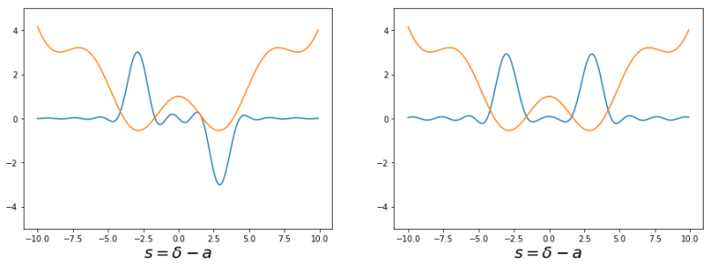
The diagram shows the ground state (blue curve on the left hand side) and the first excited state (blue curve on the right hand side). In both diagrams, I have added the classical potential (orange line) for the purpose of comparison. So we actually obtain the picture that we expect. Up to normalization, the ground state – the eigenstate on the left – is a superposition of two states

where is a state localized around the left minimum of the potential and is a state centered around the right minimum, whereas the first excited state is a linear combination proportional to

In general, there will be a small energy difference between these two states, which leads to a non-zero probability for tunneling between them. Intuitively, the state corresponds to a supercurrent that flows through the loop in one direction and the state is a state in which the supercurrent flows in the opposite direction. Our ground state – which would be the state in an interpretation as a qubit – and our first excited state are superpositions of these two states.

A nice property of the flux qubit is that the energy gap between the first excited state and the second excited state is much higher than the energy gap between the ground state and the first excited state. In the example used as basis for the numerical simulations described here, the second gap is more than one order of magnitude higher than the first gap. This implies that the two level system spanned by and is a fairly well isolated system and thus serves as a very good approximation to a qubit. The Hamiltonian can be manipulated by changing the flux through the loop by applying an external magnetic field or an external microwave pulse can be used to stimulate a transition from the ground state to the first excited state. In this way, the qubit can be read-out and controlled.

So theoretically, this system is a good candidate for the implementation of a qubit. In fact, this has been used in practice – the D-Wave quantum annealer is based on interconnected flux qubits. However, it seems that the flux qubit has come a bit out of fashion, and research has focussed on a new generation of superconducting qubits like the transmon qubit that work slightly differently. We will study this type of qubit in the next post in this series.