During the second half of the last decade, researchers have started to exploit the impressive capabilities of graphical processing units (GPUs) to speed up the execution of various machine learning algorithms (see for instance [1] and [2] and the references therein). Compared to a standard CPU, modern GPUs offer a breathtaking degree of parallelization – one of NVIDIAs current flagships, the Tesla V100, offers more than 5.000 CUDA cores that can perform work in parallel. As training and evaluating neural networks involves many floating operations on large matrices, they can benefit heavily from the special capabilities that a GPU provides.
So how can we make our code execute on a GPU? Of course you could program directly against the CUDA interface or similar interfaces like OpenCL. But specifically for the purposes of machine learning, there are easier options – over the last years, several open source frameworks like Theano, Torch, MXNet or TensorFlow have become available that make it comparatively easy to leverage a GPU for machine learning. In this post, I will use the TensorFlow framework, simply because so far this is the only one of these frameworks that I have used (though MXNet looks very interesting too and I might try that out and create a post on it at some point in the future).
It takes some time to get used to the programming model of TensorFlow which is radically different from the usual imparative programming style. As an example, let us suppose we wanted to add two matrices. In Python, using numpy, this would look as follows.
import numpy as np
a = np.matrix([[0, 1], [1, 0]])
b = np.matrix([[1, 0], [0, 1]])
c = a + b
print(c)
This program is described by a sequence of instructions (let us ignore the fact for a moment that these are of course functions that we call – ultimately, functions are composed of instructions). When we execute this program, the instructions are processed one by one. First, we assign a value to the variable a, then we assign a value to a variable b, then we add these two values and assign the result to a variable c and finally we print out the value of c.
The programming model behind TensorFlow (and other frameworks like Theano) is fundamentally different. Instead of describing a program as a sequence of instructions, the calculations are organized as a graph. The nodes in this graph correspond to operations. The edges joining the nodes represent the flow of data between the operations. In TensorFlow, data is always represented as a tensor, so the edges in the graph are tensors. An operation consumes data from its inputs, processes it and forwards it to the next operation in the graph as its output.
A program using TensorFlow typically consists of two phases. In the first phase, we build the graph, i.e. we define the operations and their inputs and outputs that make up the calculation that we want to perform. However, in this phase, no calculations are actually performed. Instead, this happens in the second phase when we actually run the graph. For that purpose, we create a session. Roughly speaking, a session defines an environment in which a graph can be executed. Once the session has been defined, we can invoke its run method. To the run method, we pass as an argument the operation in the graph that we want to execute. The run method will then trace the graph backwards and evaluate all operations that provide input to our target operation recursively, i.e. it will identify the subgraph that needs to be executed to evaluate our target operation.
Let us again use the example of a simple addition to illustrate this. The source code looks as follows.
import tensorflow as tf
#
# Build the model
#
a = tf.constant([[0, 1], [1, 0]], name="a")
b = tf.constant([[1, 0], [0, 1]], name="b")
c = tf.add(a,b, name="c")

#
# Create a session and run it
#
session = tf.Session()
print(session.run(c))
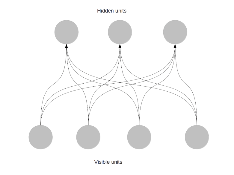
First, we import the tensorflow library itself. Then, in the next three lines, we build the graph. We define three nodes in the graph. The first two nodes are special operations that output simply a constant value. The third operation is the operation that performs the actual addition and uses the previously defined operations as input. Thus our final graph has three nodes and two edges, as shown below.h

In the next line, we create a TensorFlow session which we then run. The argument specifies which operation we want to execute and therefore determines which part of the graph we will actually run. The output of the run method is an ordinary numpy array which we then print out.
Let us now look at an example which is slightly more complicated. In the PCD algorithm, we can compute the contribution of the negative phase to the weight updates as follows.
E = expit(self.beta*(np.matmul(S0, self.W) + self.c))
pos = np.tensordot(S0, E, axes=((0),(0)))
Here S0 is a batch from the sample set, W is the current value of the weights and c is the current value of the bias. In TensorFlow, the code to build the corresponding part of the model looks quite similar.
S0 = tf.placeholder(name="S0", shape=[batch_size, self.visible],
                    dtype=tf.float32)
W = tf.get_variable(name="W",
                        dtype=tf.float32,
                        shape=[self.visible, self.hidden],
                        initializer = tf.zeros_initializer(),
                        trainable=False)
c = tf.get_variable(name="c",
                        dtype=tf.float32,
                        shape=[1, self.hidden],
                        initializer = tf.zeros_initializer(),
                        trainable=False)
E = tf.sigmoid(self.beta*(tf.matmul(S0, W) + c), name="E")
pos = tf.tensordot(S0, E, axes=[[0],[0]], name="pos")
The first element that we define – S0 – is a so called placeholder. This is a bit like a constant, with the difference that its value can be specified per run, using an additional argument called feed dictionary to the Session.run method. The next two elements that we define are variables. Variables are similar to operations – they represent nodes in the network and provide an output, but have no input. Instead, they have a certain value and feed that value as outputs to other operations. We then use the built-in tensorflow operations sigmoid and tensordot to calculate the expectation values of the visible units and the positive phase.
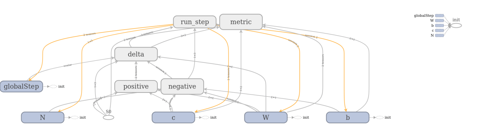
The full model to train a restricted Boltzmann machine is of course a bit more complicated. TensorFlow comes with a very useful device called TensorBoard that can be used to visualize a graph constructed in TensorFlow. The image below has been created using TensorFlow and shows the full graph of our restricted Boltzmann machine.
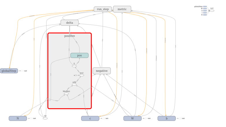
TensorBoard offers the option to combine operations into groups which are then collapsed in the visual representation. In the image above, all groups are collapsed except the group representing the contribution from the positive phase. We can clearly see the flow of data as described above – we first multiply S0 and W, then add c to the result, multiply this by a constant (the inverse temperature, called x in the diagram) and then apply the sigmoid operation that we have called E. The result is then fed into other, collapsed groups like the group delta which holds the part of the model responsible for calculating the weight updates.
I will not go through the full source code that you can find on GitHub as usual – you will probably find the well written tutorial on the TensorFlow homepage useful when going through this. Instead, let us play around a bit with the result.
As the PC that is under my desk is almost seven years old and does not have a modern GPU, I did use a p2.xlarge instance from Amazon EC2 which gave me access to a Tesla K80 GPU and four Intel Xeon E5-2686 cores running at 2.3 GHz (be careful – this instance type is not covered by the free usage tier, so that will cost you a few dollars). I used the Amazon provided Deep Learning AMI based on Ubuntu 16.04. After logging into the instance, we first have to complete a few preparational steps.
$ source activate tensorflow_p36
$ git clone http://www.github.com/christianb93/MachineLearning.git
$ cd MachineLearning
$ export MPLBACKEND="AGG"
$ conda install scikit-learn
$ python3 RBM.py --algorithm=PCDTF
Here we activate the pre-configured TensorFlow environment, download the source code from GitHub, set the environment variable to define our Matplotlib backend, and download and install some required packages. Then we do a first run with the BAS dataset to verify that everything works. If that is the case, we can run the actual MNIST training and sampling.
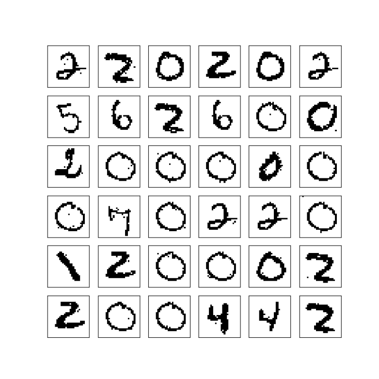
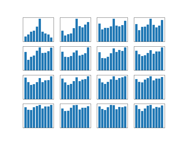
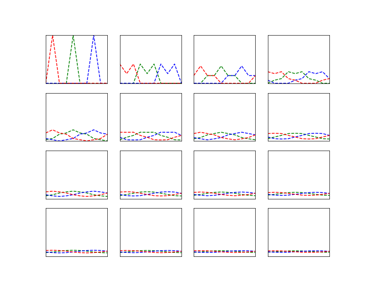
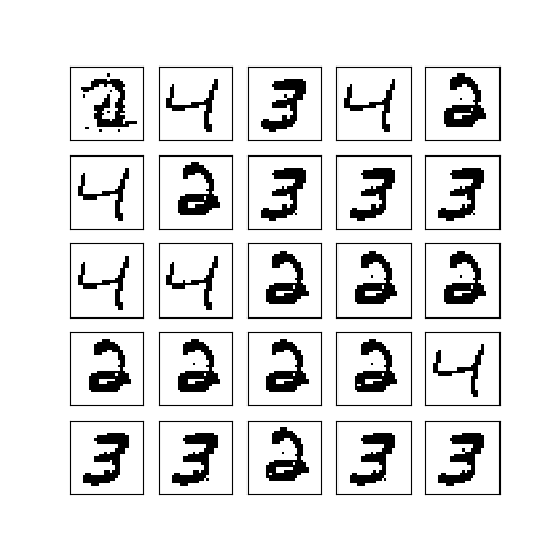
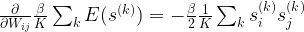
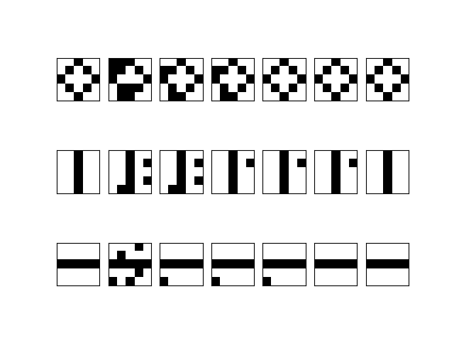
$ python3 RBM.py --N=28 --data=MNIST --save=1 --hidden=128 --pattern=256 --batch_size=128 --epochs=40000 --run_samples=1 --sample_size=6,6 --beta=1.0 --sample=200000 --algorithm=PCDTF --precision=32
This produced the following sample of 6 x 6 digits.
The execution took roughly 5 minutes – 2 minutes for the training phase and 3 minutes for the sampling phase. During the training, the GPU utilization (captured with nvidia-smi -l 2) was at around 57% and stayed in that range during the sampling phase.
A second run using the switch --precision=64 to set the floating point precision to 64 bits did not substantially change the outcome or the performance.
Then a run with the same parameters was done in pure Python running on the four CPU cores provided by the p2.xlarge instance (--algorithm=PCD). During the training phase, the top command showed a CPU utilization of 400%, i.e. all four cores where at 100%. The utilization stayed in that range during the sampling phase. The training took 10:20 minutes, the sampling 8 minutes. Thus the total run time was 18 minutes compared to 5 minutes – a factor of 360%.
Following the advice on this post, I then played a bit with the settings of the GPU and adjusted the clock rates and the auto boost mode as follows.
sudo nvidia-smi --auto-boost-default=0
sudo nvidia-smi -ac 2505,875
That brought the GPU utilization down to a bit less than 50%, but had a comparatively small impact on the run times which now were 1:40 min (instead of 2 min) for training and 2:30 min (instead of 3 min) for sampling. So the total run time was now a bit more than 4 minutes, which is a speed up of roughly 20% compared to the default settings. Compared to the CPU, we have now reached a speed up of almost 4,5.
Next, let us compare this to the run time on two CPUs only. To measure that, I grabbed an instance of the t2.large machine type that comes with 2 CPUs – according to /proc/cpuinfo, it is equipped with two Intel Xeon E5-2676 CPUs at 2.40GHz. Interestingly, the training phase only took roughly 8 minutes on that machine, which is even a bit faster than on the p2.xlarge which has four cores. The sampling phase was faster as well, taking only 6 minutes instead of 8 minutes. It seems that adding more CPUs increases the overhead for the synchronisation between the cores drastically so that it results in a performance penalty instead of a performance improvement. To verify this, I did a run on a p2.8xlarge with 32 CPUs and got a similar result – training took 9 minutes, sampling 6:50 minutes.
Finally, I could not resist the temptation to try this out on a more advanced GPU enabled machine. So I got a p3.2xlarge instance which contains one of the relatively new Tesla V100 GPUs. I did again adjust the application clocks using
sudo nvidia-smi -ac 877,1530
With these settings, one execution now took only about 1:20 minutes for the training and 1:50 min for the sampling. However, the GPU utilization was only at 30% – so we have reached a point where just having a faster GPU does not lead to a significant speed advantage any more. The following table summarizes the results of the various measurements.
| Instance |
Run time training |
Run time sampling |
| p3.2xlarge (Tesla V100) |
1:20 min |
1:40 min |
| p2.large (Tesla K80) |
1:40 min |
2:30 min |
| p2.large (4 x CPU) |
10 min |
8 min |
| p2.8xlarge (32 x CPU) |
9 min |
6:50 min |
| t2.large (2 x CPU) |
8 min |
6 min |
Of course we could now start to optimize the implementation. For the training phase, I assume that the bottleneck that limits GPU utilization is the use of the feed dictionary mechanism which could be replaced by queues to avoid overhead of switching back between CPU and GPU. During the sampling phase, we could also try to reduce the relative overhead of the run method by combining a certain number of steps – say 10 – into the graph and thus reducing the number of iterations that happen outside of the model. It would be interesting to play with this and see whether we can improve the performance significantly. But this is already a long post, so I will leave this for later…
References
1. R. Raina, A. Madhavan, A. Ng, Large-scale Deep Unsupervised Learning using Graphics Processors, Proceedings of the 26 th International Conference on Machine Learning (2009)
2. K. Chellapilla, S. Puri , P. Simard, High Performance Convolutional Neural Networks for Document Processing, International Workshop on Frontiers in Handwriting Recognition (2006)


 where N is the number of states. We also assume that all our points are measurable, i.e we consider our state space as a discrete probability space.

 of random variables taking values in X with the Markov property saying that for all times t, the conditional distribution for Xt+1 given all previous values
  only depends on Xt, i.e.
 . We can think of the combined values
  for all times t as a history of states or as a random walk in the state space. The Markov property then means that the probability to transition into a next state does not depend on the full history, but only on the current state – Markov chains do not have a memory.
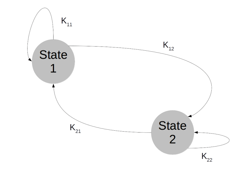
 . What is the probability to be in state j after one step? Of course we can write


 .
.

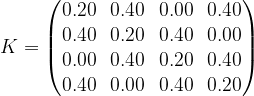
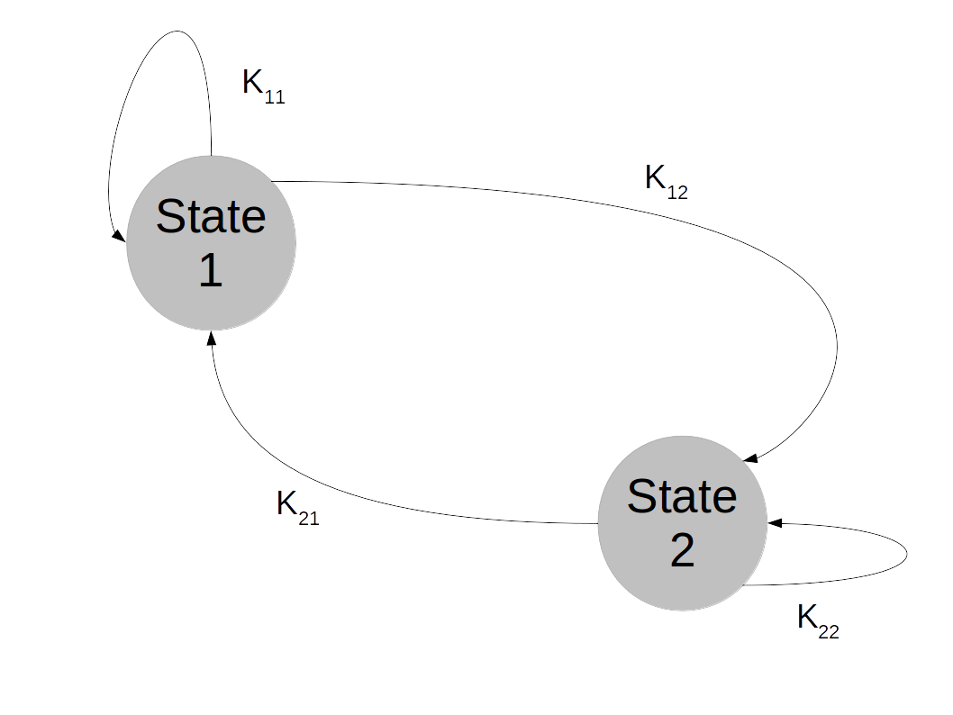
 , then the transition matrix is given by a matrix of the form (for instance for N=4)


 . If we take

![\Delta W_{ij} = \beta \left[ \langle v_i \sigma(\beta a_j) \rangle_{\mathcal D} - \langle v_i \sigma(\beta a_j) \rangle_{P(v)} \right]](https://s0.wp.com/latex.php?latex=%5CDelta+W_%7Bij%7D+%3D+%5Cbeta+%5Cleft%5B+%5Clangle+v_i+%5Csigma%28%5Cbeta+a_j%29+%5Crangle_%7B%5Cmathcal+D%7D+-+%5Clangle+v_i+%5Csigma%28%5Cbeta+a_j%29+%5Crangle_%7BP%28v%29%7D+%5Cright%5D++&bg=FFFFFF&fg=000&s=1&c=20201002)
 that appears several times is simply the conditional probability for the hidden unit j to be “on” and, as only the values 0 and 1 are possible, at the same time the conditional expectation value of that unit given the values of the visible units – let us denote this quantity by
  . Our update rule now reads
![\Delta W_{ij} = \beta \left[ \langle v_i e_j \rangle_{\mathcal D} - \langle v_i e_j \rangle_{P(v)} \right]](https://s0.wp.com/latex.php?latex=%5CDelta+W_%7Bij%7D+%3D+%5Cbeta+%5Cleft%5B+%5Clangle+v_i+e_j+%5Crangle_%7B%5Cmathcal+D%7D+-+%5Clangle+v_i+e_j+%5Crangle_%7BP%28v%29%7D+%5Cright%5D++&bg=FFFFFF&fg=000&s=1&c=20201002)
 after each step and take the average of these values.
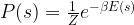
 with probability
  with probability

![W = W + \lambda \beta \left[ v e^T - \bar{v} \bar{e}^T \right]](https://s0.wp.com/latex.php?latex=W+%3D+W+%2B+%5Clambda+%5Cbeta+%5Cleft%5B+v+e%5ET+-+%5Cbar%7Bv%7D+%5Cbar%7Be%7D%5ET+%5Cright%5D+&bg=FFFFFF&fg=000&s=0&c=20201002)
![b = b + \lambda \beta \left[ v - \bar{v} \right]](https://s0.wp.com/latex.php?latex=b+%3D+b+%2B+%5Clambda+%5Cbeta+%5Cleft%5B+v+-+%5Cbar%7Bv%7D+%5Cright%5D+&bg=FFFFFF&fg=000&s=0&c=20201002)
![c = c + \lambda \beta \left[ e - \bar{e} \right]](https://s0.wp.com/latex.php?latex=c+%3D+c+%2B+%5Clambda+%5Cbeta+%5Cleft%5B+e+-+%5Cbar%7Be%7D+%5Cright%5D+&bg=FFFFFF&fg=000&s=0&c=20201002)
 is then the contribution of the negative phase to the update of
  . We can summarize the contributions for all pairs of indices as the matrix
  . Similarly, the positive phase contributes with
  . In the next line, we update W with both contributions, where
  is the learning rate. We then apply similar update rules to the bias for visible and hidden units – the derivation of these update rules from the expression for the likelihood function is done similar to the derivation of the update rules for the weights as shown in my last post.
 is set to 2.0. In each iteration, a mini-batch of 10 patterns is trained.
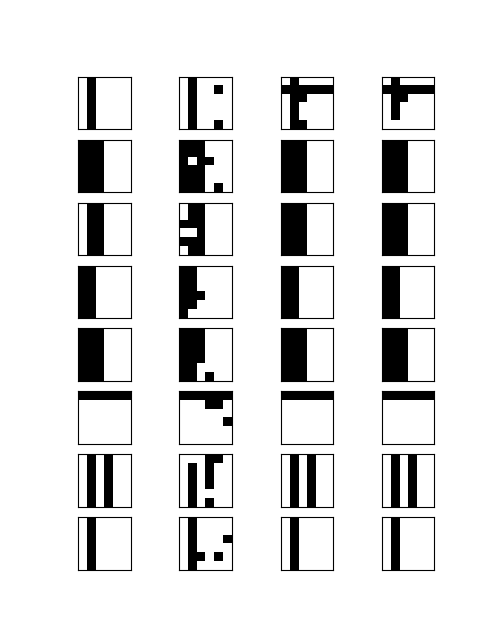


 and a hidden unit if i is in the set
  . Second, it is common to use 0 and 1 as states instead of -1 and +1. Our state space then splits


 is the k-the sample point corresponding to a set of values for the visible units.
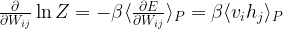


![\Delta W_{ij} = \lambda \beta \left[ \langle \langle v_i h_j \rangle_{P(\cdot | v)} \rangle_{\mathcal D} - \langle v_i h_j \rangle_P \right]](https://s0.wp.com/latex.php?latex=%5CDelta+W_%7Bij%7D+%3D+%5Clambda+%5Cbeta+%5Cleft%5B+%5Clangle+%5Clangle+v_i+h_j+%5Crangle_%7BP%28%5Ccdot+%7C+v%29%7D+%5Crangle_%7B%5Cmathcal+D%7D+-+%5Clangle+v_i+h_j+%5Crangle_P+%5Cright%5D++&bg=FFFFFF&fg=000&s=1&c=20201002)


 to be one given v, so that this turns into

 in this way and then ignoring the values of the hidden units in this way gives a sampler for the marginal distribution.


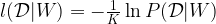
![s^{(k]}](https://s0.wp.com/latex.php?latex=s%5E%7B%28k%5D%7D&bg=FFFFFF&fg=000&s=0&c=20201002) . Assuming that the sample states are independent, we can write the probability for the data given the weights W as the product.
. Assuming that the sample states are independent, we can write the probability for the data given the weights W as the product.

 is the k-th sample point, where we assume that all sample points are drawn independently.


![\frac{\partial}{\partial W_{ij}} l({\mathcal D} | W) = - \frac{\beta}{2} \left[ \langle s_i s_j \rangle_{\mathcal D} - \langle s_i s_j \rangle_P \right]](https://s0.wp.com/latex.php?latex=%5Cfrac%7B%5Cpartial%7D%7B%5Cpartial+W_%7Bij%7D%7D+l%28%7B%5Cmathcal+D%7D+%7C+W%29+%3D+-+%5Cfrac%7B%5Cbeta%7D%7B2%7D+%5Cleft%5B+%5Clangle+s_i+s_j+%5Crangle_%7B%5Cmathcal+D%7D+-+%5Clangle+s_i+s_j+%5Crangle_P+%5Cright%5D++&bg=FFFFFF&fg=000&s=1&c=20201002)
![\Delta W_{ij} = \frac{1}{2} \lambda \beta \left[ \langle s_i s_j \rangle_{\mathcal D} - \langle s_i s_j \rangle_P \right]](https://s0.wp.com/latex.php?latex=%5CDelta+W_%7Bij%7D+%3D+%5Cfrac%7B1%7D%7B2%7D+%5Clambda+%5Cbeta+%5Cleft%5B+%5Clangle+s_i+s_j+%5Crangle_%7B%5Cmathcal+D%7D+-+%5Clangle+s_i+s_j+%5Crangle_P+%5Cright%5D++&bg=FFFFFF&fg=000&s=1&c=20201002)
 across all sample points, i.e. we strengthen a connection between two units if the two units are strongly correlated in the sample set, and weaken the connection otherwise. The second term is a correction to the Hebbian rule that does not appear in a Hopfield network.


 patterns, where N is the number of units. In our case, with 25 units, this would be approximately 3 to 4 patterns.
 .
. is the strength of the connection between the units i and j. We assume that no neuron is connected to ifself, i.e. that
  , and that the matrix of weights is symmetric, i.e. that
  .
.

 . Let
. Let


 and the activation of unit i is never negative, this implies that during the upgrade process, the energy function will always increase or stay the same. Thus the state will settle in a local minimum of the energy function.

 are the states that the network should remember (in a later post in this series, we will see that this rule can be obtained as the low temperature limit of a training algorithm called contrastive divergence that is used to train a certain class of Boltzmann machines).
 and
and  have the same sign, i.e. are in the same state. This corresponds to a rule known as Hebbian learning rule that has been postulated as a principle of learning by D. Hebb and basically states that during learning, connections between neurons are enforced if these neurons fire together (