
In the last post, we have seen how we can implement and train an RNN on a very simple task – learning how to count. In the example, I have chosen a sequence length of L = 6. It is tempting to play around with this parameter to see what happens if we increase the sequence length.
In this notebook, I implemented a very simple measurement. I did create and train RNNs on a slightly different task – remembering the first element of a sequence. We can use the exact same code as in the last post and only change the line in the dataset which prepares the target to
targets = torch.tensor(self._L*[index], dtype=torch.long)
I also changed the initialization approach compared to our previous post by using a random uniform distribution, similar to what PyTorch is doing. I then did training runs for different values of the sequence length, ranging from 4 to 20, and measured the accuracy on the training set after each training run.
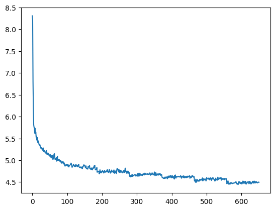
The blue curve in the diagram below displays the result, showing the sequence length on the x-axis and the accuracy on the y-axis (we will get to the meaning of the upper curve in a second).
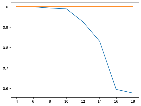
Clearly, the efficiency of the network decreases with larger sequence length, starting at a sequence length of approximately 10, and accuracy drops to less than 60%. I also repeated this with our custom build RNN replaced by PyTorchs RNN to rule out issues with my code, and got similar results.
This seems to indicate that there is a problem with higher sequence lengths in RNNs, and in fact there is one (you might want to take a look at this paper for a more thorough study, which, however, arrives at a similar result – RNNs have problems to learn dependencies in time series with a range of more than 10 or 12 time steps). Given that our task is to simply remember the first item, it appears that an RNNs memory is more of a short-term memory and less of a long term memory.
The upper, orange curve looks much more stable and maintains an accuracy of 100% even for long sequences, and in fact this curve has been generated using a more advanced network architecture called LSTM, which is the topic of todays post.
Before we explain LSTMs, let us try to develop an intuition what the problem is they are trying to solve. For that purpose, it helps to look at how backpropagation actually works for RNNs. Recall that in order to perform automatic differentiation, PyTorch (and similar frameworks) build a computational graph, starting at the inputs and weights and ending at the loss function. Now look at the forward function of our network again.
for t in range(L):
  h = torch.tanh(x[t] @ w_ih.t() + b_ih + h @ w_hh.t() + b_hh)
  out.append(h)
Notice the loop – in every iteration of the loop, we continue our calculation, using the values of the previous loop (the hidden layer!) as one of the inputs. Thus we do not create L independent computational graphs, but in fact one big computational graph. The depth of this graph grows with larger L, and this is where the problem comes from.
Roughly speaking, during backpropagation, we need to go back the entire graph, so that we move “backwards in time” as well, going back through all elements of the graph added during each loop iteration (this is why this procedure is sometimes called backpropagation in time). So the effective length of the computational graph corresponds to that of a deep neural network with L layers. And we therefore face one of the problems that these networks have – vanishing gradients.
In fact, when we run the backpropagation algorithm, we apply the chain rule at least once for every time step. The chain rule involves a multiplication by the derivative of the activation function. As these derivatives tend to be smaller than one, this can, in the worst case, imply that the gradient gets smaller and smaller with each time step, so that eventually the error signal vanishes and the network stops learning. This is the famous vanishing gradient problem (of course this is by no means a proof that this problem really occurs in our case, however, this is at least likely, as it disappears after switching to an LSTM, so let us just assume that this is really the case….).
So what is an LSTM? The key difference between an LSTM and an ordinary RNN is that in addition to the hidden state, there is a second element that allows the model to remember information across time steps called the memory cell c. At time t, the model has access to the hidden state from the previous time step and, in addition, to the memory cell content from the previous time step, and of course there is an input x[t] for the current time step, like a new word in our sequence. The model then produces a new hidden state, but also a new value for the memory cell at time t. So the new value of the hidden state and the new value of the cell are a function of the input and the previous values.

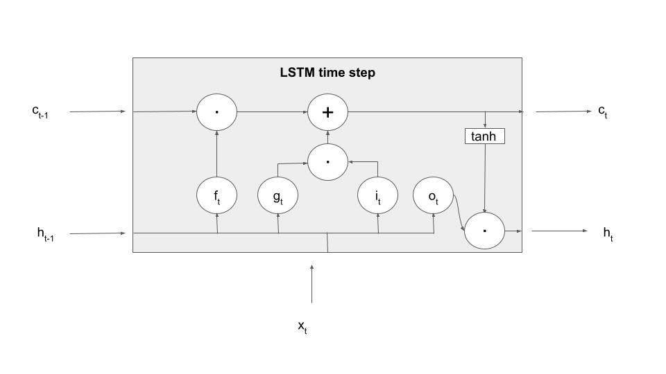
Here is a diagram that displays a single processing step of an LSTM – we fill in the details in the grey box in a minute.
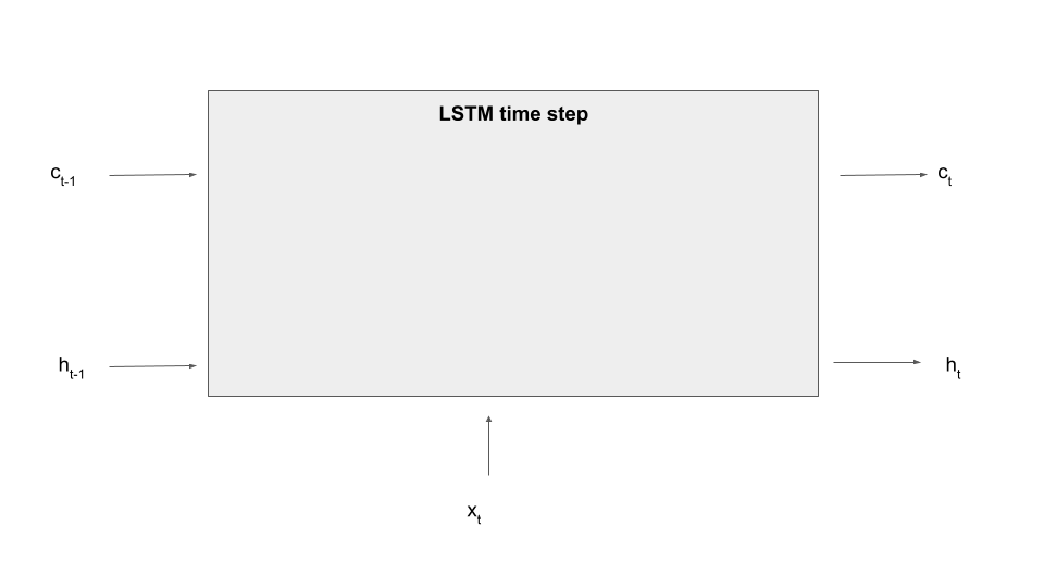
So far this is not so different from an ordinary RNN, as the memory cell is treated similarly to a hidden layer. The key difference is that a memory cell is gated, which simply means that the cell is not directly connected to other parts of the network, but via learnable matrices which are called gates. These gates determine what content present in the cell is made available to the current time step (and thus subject to the flow of gradients during backward processing) and which information is kept back and used either not at all or during the next time step. Gates also control how new information, i.e. parts of the current input, are fed into the cells. In this sense, the memory cell acts a as more flexible memory, and the network can learn rules to erase data in the cell, add data to the cell or use data present in the cell.
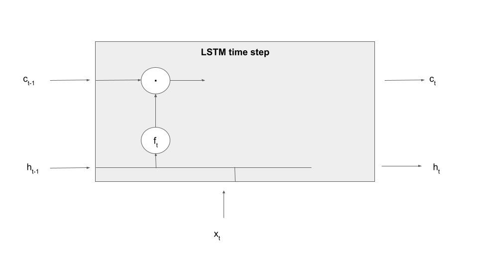
Let us make this a bit more tangible by explaining the first processing step in an LSTM time step – forgetting information present in the cell. To realize this, an LSTM contains an additional set of weights and biases that allow it to determine what information to forget based on the current input and the previous value of the hidden layer, called (not surprisingly) the input-forget weight matrix Wif, the input-forget bias bif, and similarly for Whf and bhf. These matrices are then combined with inputs and hidden values and undergo a sigmoid activation to form a tensor known as the forget gate.

In the next step, this gate is multiplied element-wise with the value of the memory cell from the previous time step. Thus, if a dimension in the gate f is close to 1, this value will be taken over. If, however, a dimension is close to zero, the information in the memory cell will be set to zero, will therefore not be available in the upcoming calculation and in the output and will in that sense be forgotten once the time step completes. Thus the tensor f controls which information the memory cell is supposed to forget, explaining its name. Expressed as formula, we build

Let us add this information to our diagram, using the LaTex notation (a circle with a dot inside) to indicate the component-wise product of tensors, sometimes called the Hadamard-Product.
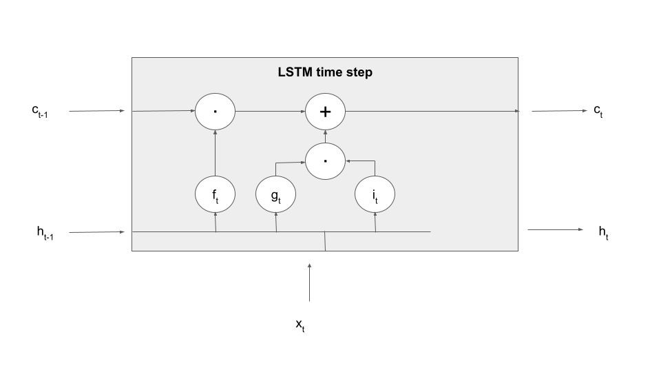
The next step of the calculation is to determine what is sometimes called the candidate cell, i.e. we want to select data derived from the input and the previous hidden layer that is added to the memory cell and thus remembered. Even though I find this a bit confusing I will instead follow the convention employed by PyTorch and other sources to use the letter g to denote this vector and call it the cell gate (the reason I find this confusing is that it is not exactly a gate, but, as we will see in a minute, input that is passed through the gate into the cell). This vector is computed similarly to the value of the hidden layer in an ordinary RNN, using again learnable weight matrices and bias vectors.

However, this information is not directly taken over as next value of the memory cell. Instead, a second gate, the so-called input gate is applied. Then the result of this operation is added to the output of the forget gate times the previous cell value, so that the new cell value is now the combination of a part that survived the forget-gate, i.e. the part which the model remembers, and the part which was allowed into the memory cell as new memorizable content by the input gate. As a formula, this reads as


Let us also update our diagram to reflect how the new value of the memory cell is computed.
We still have to determine the new value of the hidden layer. Again, there is a gate involved, this time the so-called output gate. This gate is applied to the value of the tanh activation function on the new memory cell value to form the output value, i.e.

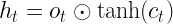
Adding this to our diagram now yields a complete picture of what happens in an LSTM processing step – note that, to make the terminology even more confusing, sometimes this entire box is also called an LSTM cell.
This sounds complicated, but actually an implementation in PyTorch is more straighforward than you might think. Here is a simple forward method for an LSTM. Note that in order to make the implementation more efficient, we combine the four matrices Wif, Wig, Wio and Wii into one matrix by concatenating them along the first dimension, so that we only have to multiply this large matrix by the input once, and similarly for the hidden layer. The convention that we use here is the same that PyTorch uses – the input gate weights come first, followed by the forget gate, than the cell gate and finally the output gate.,
def forward(x):
    L = x.shape[0]
    hidden = torch.zeros(H)
    cells = torch.zeros(H)
    _hidden = []
    _cells = []
    for i in range(L):
        _x = x[i]
        #
        # multiply w_ih and w_hh by x and h and add biases
        #
        A = w_ih @ _x
        A = A + w_hh @ hidden
        A = A + b_ih + b_hh
        #
        # The value of the forget gate is the second set of H rows of the result
        # with the sigmoid function applied
        #
        ft = torch.sigmoid(A[H:2*H])
        #
        # Similary for the other gates
        #
        it = torch.sigmoid(A[0:H])
        gt = torch.tanh(A[2*H:3*H])
        ot = torch.sigmoid(A[3*H:4*H])
        #
        # New value of cell
        # apply forget gate and add input gate times candidate cell
        #
        cells = ft * cells + it * gt
        #
        # new value of hidden layer is output gate times cell value
        #
        hidden = ot * torch.tanh(cells)
        #
        # append to lists
        #
        _cells.append(cells)
        _hidden.append(hidden)
    return torch.stack(_hidden)
In this notebook, I have implemented this (with a few tweaks that allow the processing of previous values of hidden layer and cell, as we have done it for RNNs) and verified that the implementation is correct by comparing the outputs with the outputs of the torch.nn.LSTM class which is the LSTM implementation that comes with PyTorch.
The good news it that even though LSTMs are more complicated than ordinary RNNs, the way they are used and trained is very much the same. You can see this nicely in the notebook that I have used to create the measurements presented above – using an LSTM instead of an RNN is simply a matter of changing one call, all the other parts of the data preparation, training loop and inference remain the same. This measurement also shows that LSTMs do in fact achieve a much better performance when it comes to detecting long-range dependencies in the data.
LSTMs were first proposed in this paper by Hochreiter and Schmidhuber in 1997. If you consult this paper, you will find that this original version did in fact not contain the forget gate, which was added by Gers, Schmidhuber and Cummins three years later. Over time, other versions of LSTM networks have been developed, like the GRU cell.
Also note that LSTM layers are often stacked on top of each other. In this architecture, the hidden state of an LSTM layer is not passed on directly to an output layer, but to a second LSTM layer, playing the role of the input from this layers point of view.
I hope that this post has given you an intuition for how LSTMs work. Even if our ambition is mainly to understand transformers, LSTMs are still relevant, as the architectures that we will meet when discussing transformers like encoder-decoder model and attention layers, and training methods like teacher forcing have been developed based on RNNs and LSTMs .
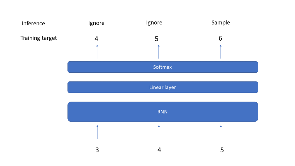
There is one last ingredient that we will need to start working on our first project – sampling, i.e. using the output of a neural network to create the next token or word in a sequence. So far, our approach to this has been a bit naive, as we just picked the token with the highest probability. In the next post, we will discuss more advanced methods to do this.


 , in practice this could be weights, bias terms or any other parameters. To simplify things a bit, we will also assume that the latent variable is finite. Our aim is to maximize the log likelihood, which we can – under these assumptions – express as follows.
 . For that purpose, we introduce a term that is traditionally called Q and defined as follows (all this is a bit abstract, but will become clearer later when we do an example):
![Q(\Theta'; \Theta) = E \left[ \ln P(x,z | \Theta') | x, \Theta \right]](https://s0.wp.com/latex.php?latex=Q%28%5CTheta%27%3B+%5CTheta%29+%3D+E+%5Cleft%5B++%5Cln+P%28x%2Cz+%7C+%5CTheta%27%29++%7C+x%2C+%5CTheta+%5Cright%5D++&bg=FFFFFF&fg=000&s=1&c=20201002)
 of z. Thus the right hand side is, spelled out
![E \left[ \ln P(x,z | \Theta') | x, \Theta \right] = \sum_z \ln P(x,z | \Theta') P(z | x, \Theta)](https://s0.wp.com/latex.php?latex=E+%5Cleft%5B++%5Cln+P%28x%2Cz+%7C+%5CTheta%27%29++%7C+x%2C+%5CTheta+%5Cright%5D+%3D+%5Csum_z+%5Cln+P%28x%2Cz+%7C+%5CTheta%27%29+P%28z+%7C+x%2C+%5CTheta%29++&bg=FFFFFF&fg=000&s=1&c=20201002)
 of parameters such that when passing from
  to
to  , the value of Q does not decrease, i.e.

 is maximized. This part of the algorithm is therefore called the maximization step. Then we start over, using


 and
and  . Using this notation, we can now write down the result of calculating the Q function:
 . For a fixed
  and
and  , and we can now try to maximize this function with respect to these parameters. This calculation is not difficult, but again a bit tiresome (and requires the use of Lagrangian multipliers as there is a constraint on the
  ), and I again refer to


 , the covariance matrices
  and the means
  – which could, for instance, be chosen randomly. Then, we calculate the responsibilities as above – essentially, this is the expectation step, as it amounts to finding Q.
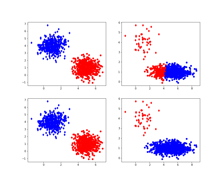
 of points in some euclidian space and a number K of clusters. We want to identify the centre
  of each cluster and then assign the data points xi to some of the
  , namely to the

 of cluster centers, we can easily minimize Rij by assigning each data point to the cluster whose center is closest to xi. Thus we set


 is a multivariate Gaussian distribution with mean
 .
. with the additional constraint that only one of the Zk is allowed to be different from zero. We interpret


 is as above and
 . As we already have k, this amounts to sampling from the Gaussian distribution
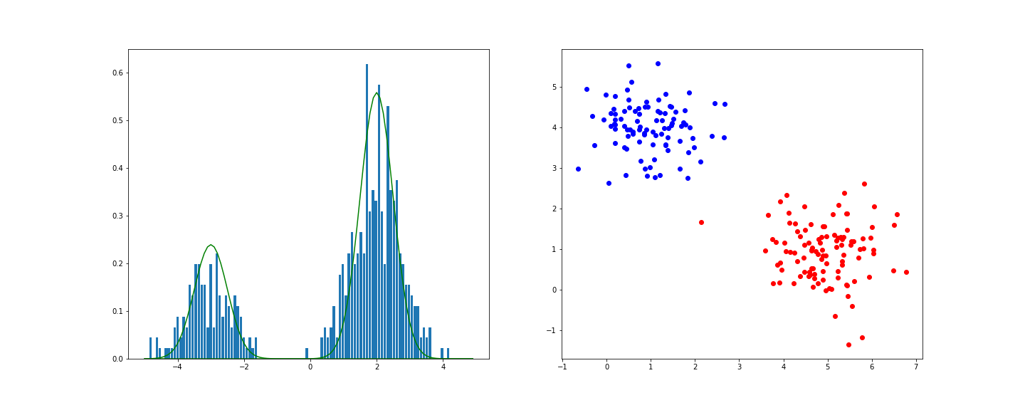


 . Another data point the network could get is

 to be a bird is a function of the Xi. In other words, using the language of conditional probabilities,
 with a vector valued random variable X. The attributes of a sample are described by the feature vector X in some subset of m-dimensional euclidian space, where m is the number of different features. In our example, m=2, as we try to classify animals based on two properties. The result of the classification is described by a random variable Y taking – for the simple case of a binary classification problem – values in
 is a function parametrized by some parameter w that we call the weights of the model. The actual value w0 of w is unknown. Based on a sample for X and Y, we then try to fit the model, i.e. we try to find a value for w such that
  models the actual conditional distribution of Y as good as possible. Once the fitting phase is completed, we can then use the model to derive predictions about objects which are not in our initial sample set.

 for a single point in the state space intractable.

 .
. 

 . We now calculate
  according to the formula above. We then accept the proposal with probability
  . If the proposal is accepted, we set xn+1 = y, otherwise we set xn+1 = xn, i.e. we stay where we are.

 with probability one. This is very similar to a random search for a global maximum – we start at some point x, choose a candidate for a point with higher value of
  with a non-zero probability. This allows the algorithm to escape a local maximum much better. Intuitively, the algorithm will still try to spend more time in regions with large values of
 and
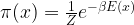
and  ) approximated using the partial sums develops over time. We see that even though we still have huge spikes, the integral remains comparatively stable and converges already after a few thousand iterations. Even if we run the simulation only for 1000 steps, we already get close to the actual values zero (for
  (for
(for 
 and
and  are the standard deviations of X and Y. In our case, given a lag, i.e. a number l less than the length of the chain, we can form two samples, one consisting of the points
  and the second one consisting of the points of the shifted series
  . The autocorrelation with lag l is then defined to be the correlation coefficient between these two series. In the diagram, we can see how the autocorrelation depends on the lag. We see that for a large lag, the autocorrelation becomes small, supporting our intuition that the series and the shifted series become independent. However, if we execute several simulation runs, we will also find that in some cases, the convergence of the autocorrelation is very slow, so care needs to be taken when trying to obtain a nearly independent sample from the chain.
  , we can use the conditional probability given either x1 or x2 as a proposal distribution. Thus, we first fix x2, and draw a new value for x1 from the conditional probability for x1 given the current value of x2. Then we move to this new coordinate, fix x1, draw from the conditional distribution of x2 given x1 and set the new value of x2 accordingly. It can be shown (see for example