Mastering large language models – Part VIII: encoder-decoder architectures and attention

The examples for LSTMs and RNNs that we have studied so far have one feature in common – the input and the output have the same length. We have seen that this is a natural choice for tasks like creating sentences based on a given prompt or attaching labels to each word in a sentence. There are, however, tasks for which this simple architecture cannot be used as we need to create a sentence based on an input of different length. To address this class of problems, encoder-decoder architectures have been developed which we will discuss today.

A good example to illustrate the challenge is machine translation. Here, we are given a source sequence, i.e. a sequence of token (x₁, …, x_S), maybe already vectorized, as input. The objective is to create a target sequence (y₁, …, y_T) as output representing the translation of the source sentence into a target language. Typically, the length T of the target sequence differs from the length S of the source sequence, which a single LSTM cannot easily cover.

Put differently, the objective is now no longer to model conditional probabilities for the completion of a sentence, i.e. probabilities of the form

but conditional probabilities for a target sequence given the source sequence, i.e. the probability distribution

The idea behind encoder-decoder architectures is to split this task into two subtasks, each of which is taken over by a dedicated network. First, there is a network called the encoder, that translates the source sequence into a single vector (or a concatentation of multiple vectors) called the context. The idea is that this vector represents, in a form independent of the length of the source sequence, an internal representation of the source sequence that somehow captures its meaning. Then a second network, the decoder, takes over. This network has access to the context and, given the context, creates the target sequence, as indicated in the diagram below..

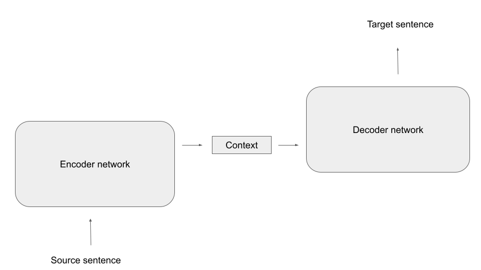
In this general form, the idea is not bound to a specific type of network. Often, encoder and decoder are both LSTMs, but we will see in a later post that also transformer networks can be used in this way.

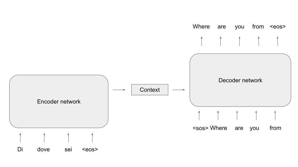
Let us now be a bit more specific on how we can bring this idea to live with LSTMs serving as decoders and encoders and specifically how these models are trained. For the encoder, this is easy – as we want the model to compress the meaning of the source sentence in the context, we of course need to feed the source sentence into the encoder. For the decoder, it is common to again apply teacher forcing. However, to create the first word of the target sentence, we need a starting point for the model. Therefore, the encoded sentences typically contain a “beginning of sentence” token, and it is also common practice to conclude the source sentence with a “end of sentence token”.

During inference, the model receives the source sequence as input and the first item of the target sequence, i.e. the beginning-of-sentence token. We can then apply any of the sampling methods discussed in an earlier post to successively generate the next word, until the model emits an end-of-sentence marker and the translation is complete.

Unfortunately, there is a fundamental problem with this architecture. If you look at the diagram, you will see that the context is the only connection between the encoder and the decoder. Consequently, the network has to compress all information necessary for the generation of the target sequence into the context, which is typically a vector of fixed size. Especially for longer source sentences, this quickly creates a bottleneck.

In 2015, Bahdanau, Cho and Bengio proposed a mechanism called attention to solve this issue. In their paper, they describe an approach which, instead of using a fixed-length context vector shared by all time steps of the decoder, uses a time-dependent context vector.

Specifically, each time step of the decoder receives three different inputs: the decoder input x_t (which, as in the diagram above, is the previous word of the target sentence), the previous hidden state h_t-1 and, in addition, a step-specific context c_t. This context is assembled from the outputs o_s of the encoder network (these are in fact not exactly the hidden states, as the architecture proposed here uses a so-called bidirectional RNN as encoder, but let us ignore this for the time being). More precisely, each context vector c_t is a weighted linear combination

of all outputs of the encoder network at all time steps. Thus, each decoder step has access to the full output of the encoder. However, and this is the crucial point, the way how the weights are calculated is governed by learned parameters which the network can adapt during training. This allows the decoder to focus on specific parts of the input sequence, depending on the current time step, i.e. to put more attention on specific time steps, lending the mechanism its name. Or, as the original paper puts it nicely in section 3.1:

“The decoder decides parts of the source sentence to pay attention to. By letting the decoder have an attention mechanism, we relieve the encoder from the burden of having to encode all information in the source sentence into a fixed length vector.“

To illustrate this, the authors include some examples for the weights used by the network. Let us look at the first of them, which illustrates the weights while translating the english sentence “The agreement on the European Economic Area was signed in 1992.”

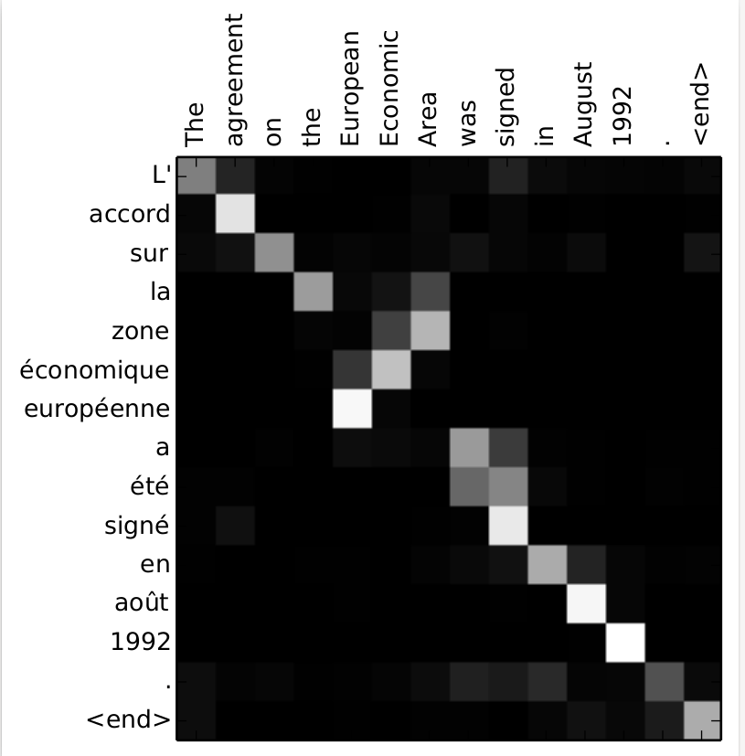
We see that, as envisioned, the network learns to focus on the word that is currently being translated, even though the order of words in target and source sentence are different.

Attention turned out to be a very powerful idea. In fact, attention is so useful that it gave rise to a new class of language models which works without the need to have a hidden state which is updated sequentially over time. This new generation of networks is called transformers, and we will start to look at transformers and at attention scores in more detail in the next post.

References:

[1] Sequence to Sequence learning with Neural Networks, Sutskever et al.
[2] Learning Phrase Representations using RNN Encoder–Decoder for Statistical Machine Translation, Cho et al.
[3] Speech and Language Processing by Jurafsky and Martin, specifically chapter 9
[4] Neural Machine Translation and Sequence-to-sequence Models by Neubig
[5] Neural Machine Translation by Jointly Learning to Align and Translate, D. Bahdanau, K.Cho, Y. Bengio