Mastering large language models – Part III: recurrent neural networks

When designing neural networks to handle language, one of the central design decisions you have to make is how you model the flow of time. The words in a sentence do not have a random order, but the order in which they appear is central to their meaning and correct grammar. Ignoring this order completely will most likely not allow a network to properly learn the structure of language.

We will later see that the transformer architecture uses a smart approach to incorporate the order of words, but before these architectures were developed, a different of models was commonly used to deal with this challenge – recurrent neural networks (RNNs). The idea of a recurrent neural network is to feed the network one word at a time, but to allow it to maintain a memory of words it has seen, or, more precisely, of their representations. This memory is called the hidden state of the model.

To explain the basic structure of an RNN, let us see how they are used to solve a very specific, but at the same time very fundamental problem – text generation. To generate text with a language model, you typically start with a short piece of text called the prompt and ask the model to generate a next word that makes sense in combination with the prompt. From a mathematical point of view, a word might be a good candidate for a continuation of the prompt if the probability that this word appears after the words in the prompt is high. Thus to build a model that is able to generate language, we train a model on conditional probabilities and, during text generation, choose the next word based on the probabilities that the model spits out. This is what large language models do at the end of the day – they find the most likely continuation of a started sentence or conversation.

Suppose, for instance, that you are using the prompt

“The”

Let us denote this word by w₁. We are now asking the model to predict, for every word w in the vocabulary, the conditional probability

$P(w | w_1)$

that this word appears after the prompt. We then sample a word according to this probability distribution, call it w₂ and again calculate all the conditional probabilities

$P(w | w_1, w_2)$

to find the next word in the sentence. We call this w₃ and so forth, until we have found a sentence of the desired length.

Let us now think about a neural network that we could use for this purpose. One approach could be an architecture similar to the one that we used for word2vec. We start with an embedding, followed by a hidden layer of a certain size (the internal dimension of the model), and add an output layer to convert back into V dimensions, were, as before, V is the size of our vocabulary.

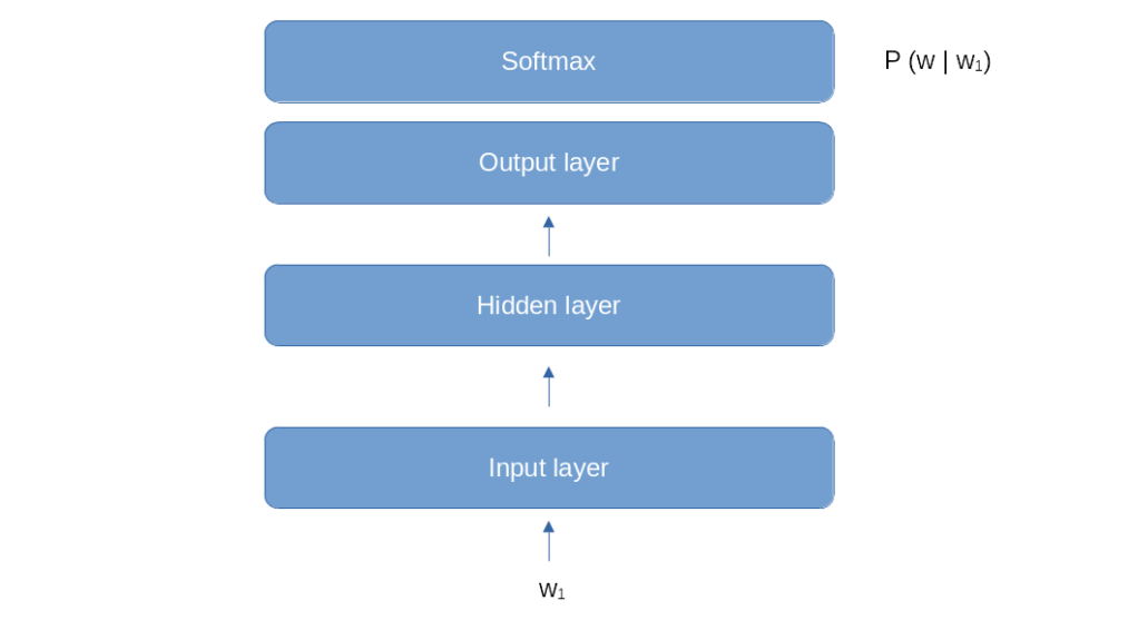
This model looks like a good fit for the first step of the word generation. If our prompt consists of one word w₁, and we need to calculate the conditional probabilities P(w | w₁), we could do this by feeding w₁ into the model and train it to predict the probabilities P(w | w₁) in its softmax layer, very much like a classical classification problem. However, things become more difficult if we have already generated two words and therefore need to calculate a conditional probability P(w | w₁, w₂) that depends on the two previous words. We could of course simply ignore w₁ and only feed w₂, which amounts to approximating

$P(w | w_1, w_2) \approx P(w | w_1)$

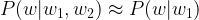
This, however, is a very crude approximation (sometimes called a unigram model), in general, the next sentence in a word will not only depend on the previous word, but on all previous words. Just think of the two sentences

Dinosaurs are big animals

Mice are small animals

If we wanted to determine the most likely word after “are”, the first word clearly does make a difference. So we need to find a way to make the previous words somehow available to our model. The approach that an RNN (or, more precisely, an Elman RNN) takes is to use a hidden layer which does not only have one input (the output of the lowest layer) but two inputs. One input is the output of the lowest layer, and the second input is the output of the hidden layer during the previous time step.

Let us go through this one by one. First, we feed word w₁ into the model as before. This goes through the input layer, through the hidden layer and finally through the output layer. However, this time, we save the output of the hidden layer and call it h₁. In the second step, we feed w₂ into the model. Again, this goes through the input layer. But now, we combine the value of the input layer with our previously saved h₁ and feed this combined value into the hidden layer to get an output h₂. We again save this, but also feed it into the output layer. In the next step, we read word w₃, combine the result of the input layer with h₂, feed this into the hidden layer and so forth. So at step t, the input the hidden layer is a function of h_t-1 (the value of the hidden layer in the previous step) and i_t (the value of the input layer at time t).

I actually found it difficult to understand this when I first read about RNNs, but sometimes code can help. So let us code this in Python. But before we do this, we need to make it more precise what it means to “combine” the value of the hidden layer from the previous time step with the value of the input layer. Combination here means essentially concatenation. More precisely, we have two weight matrices that determine the value of the hidden layer. The first matrix that we will call W_ih (the indices mean input-to-hidden) is applied to the inputs. The second one that we will call W_hh (hidden-hidden) is applied to the value of the hidden layer from the previous time step. Taking activation functions and bias into account, the value of the hidden layer at time t is therefore

$h_t = tanh(x_t W_{ih}^t + b_{ih} + h_{t-1}W_{hh}^t + b_{hh})$

where x_t is the input at time t. Note how the output from the previous step h_t-1 sneaks into this equation and realizes the feedback loop indicated in the diagram above.

Armed with this understanding, let us implement a simple RNN forward method that accepts L words (or, more generally, input vectors) and applies the above processing steps, i.e. processes L time steps.

 def forward(x):
    L = x.shape[0]
    h = torch.zeros(d_hidden)
    out = []
    for t in range(L):
        h = torch.tanh(x[t] @ w_ih.t() + b_ih + h @ w_hh.t() + b_hh)
        out.append(h)
    return torch.stack(out)

Here, d_hidden is the dimension of the hidden layer. Note that we not not include the output layer which is actually common practice (the RNN model class that comes with PyTorch does not do this either). We can clearly see that the hidden state h is saved between the individual time steps and can therefore help the model to remember information between time steps, for instance some features of the previous words that are helpful to determine the next word in the sequence.

The output of our forward function has shape (L, d_hidden), so that we have one hidden vector for every time step. We could feed this into an output layer, followed for instance by a softmax layer. Typically, however, we are only interested in the output of the last time step, which we would interpret as the conditional probability for the next word as discussed above.

Unfortunately, our forward function still has a problem. Suppose we start with a prompt with L = 3 words. We encode the words, call the forward function and obtain an output. We take the last element of the output, feed it into a feed forward layer to map back into the vocabulary, apply softmax and sample to get the next word. When we now want to determine the next word, however we would have to repeat the same procedure for the first three words to get our hidden state back that we need for the last time step. To avoid this, it would be useful if we could pass a previous hidden state as optional parameter into our model so that the forward function can pick up where it left. Similarly, we want our forward function to return the hidden layer value at the last time step as well to be able to feed it back with the next call. Here is our modified forward function.

def forward(x, h = None):
    L = x.shape[0]
    if h is None:
        h = torch.zeros(d_hidden)
    out = []
    for t in range(L):
        h = torch.tanh(x[t] @ w_ih.t() + b_ih + h @ w_hh.t() + b_hh)
        out.append(h)
    return torch.stack(out), h

This looks simple enough, but it is actually a working RNN. It is instructive to compare the output that this simple forward function produces with the output of PyTorchs torch.nn.RNN module. The GitHub repository for this series contains a simple notebook doing this, which you can again either run locally (no GPU needed) or in Google Colab using this link. This notebook also shows how to extract the weight and bias vectors from an RNN in PyTorch.

We have not yet explained how an RNN is trained. Suppose again we wanted to train an RNN for text generation. We would then pick a large corpus of text as a training dataset to obtain a large number of sentences. Each sentence would create a training sample. To force the model to predict the next word, the targets that we use to calculate the loss function are obtained by shifting the input sequence by one position to the right. If, for instance, our dataset contains the sentence “I love my cute dog”, we would turn this into a pair of inputs and targets as follows.

inputs = ["I", "love", "my", "cute"]
targets = ["love", "my", "cute", "dog"]

In particular, the target label does not depend on the prediction that the model makes during training, but only on the actual data (the “ground truth”). If, for instance, we feed the first word “I” and the model does not predict “love” but something else, we would still continue use the label “my,”, even if this does not make sense in combination with the actual model output.

This method of training is often called teacher forcing. The nice thing about this approach is that it does not require any labeled data, i.e. this is a form of unsupervised learning. The only data that we need is a large number of sentences to learn the probabilities, which we can try to harvest from public data available on the internet, like Wikipedia, social media or projects like Project Gutenberg that make novels freely available. We will actually follow this approach in a later post to train an RNN on a novel.

This concludes our post for today. In the next post, we will make all this much more concrete by implementing a toy model. This model will learn a very simple sequence, in fact we will teach the model to count, which will allow us to demonstrate the full cycle of implementing an RNN, training it using teacher forcing and sampling from it to get some results.