
In the previous post, we have discussed recurrent neural networks in the context of language processing, but in fact, they can be used to learn any type of data structured as a time series. To make sure that we really understand how this works before proceeding to more complex models, we will spent some time today and teach a simple RNN on a very specific sequence – we will teach it how to count.
As usual, this post comes with a notebook that you can either run locally (please follow the instructions in the README to set up a local environment, no GPU needed for today) or in Google CoLab using this link. So I will not go through all the details in the code, but focus on the less obvious parts of it.
First, let us discuss our dataset. Today we will in fact not ta ckle language related tasks, but simply train a model to predict the next element in a sequence. These elements are numbers between 0 and 127, and the sequences that make up our training data set are simply all sequences of six consecutive numbers in this range, like [3,4,5,6,7,8] or [56,57,58,59,60,61]. The task that the model will learn is to predict the next element in a given sequence. If, for example, we present it the sequence [3,4,5], we expect it to predict that the next element is 6.
So our dataset is really simple, the only actual work that we have to do is to convert our data items into tensors. Our input data will be one-hot encoded, so that a sequence of length L has shape (L,V) where V = 128. Our targets will just be labels, so the targets for a sequence of length L will be L labels, i.e. a tensor of shape L. Here is the code to generate an item in the dataset.
#
# Input at index is the sequence of length L
# starting at index
#
inputs = torch.arange(index, index + self._L, dtype = torch.long)
targets = torch.arange(index + 1, index + self._L + 1, dtype = torch.long)
#
# Convert inputs to one-hot encoding
#
inputs = torch.nn.functional.one_hot(inputs, num_classes = self._V)
inputs = inputs.to(torch.float32)
Next, let us discuss our model. The heart of the model will of course be an RNN. The input dimension will be V, as we plan to present the input as one-hot encoded vectors. We have already seen the forward function of the RNN in the last blog post, and it is not difficult to put this into a class that is a torch.nn.Module. Keep in mind, however, that the weights need to be wrapped into instances of torch.nn.Parameter so that they are detected by the optimizer during learning.
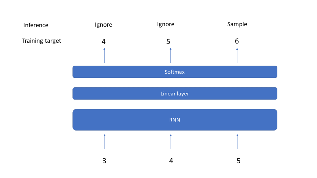
The output of the RNN will be the output of the hidden layer and will be of shape (L,D), where L is the length of the input sequence and D is the inner dimension of the model. To predict the next elements of the sequence from this, we add a linear layer that maps this back into a tensor of shape (L, V). We then take the last element of the output, which is a tensor of shape V, and apply a softmax to get a probability distribution. To make a prediction, we could now either sample according to this multinomial distribution, or just take the element with the highest probability weight – we will discuss more advanced sampling methods in a later post.
So here is the code for our model – note that we again allow a previous hidden layer value to be used as optional input.
class MyModel(torch.nn.Module):

  def __init__(self, d_in, d_hidden):
    self._d_hidden = d_hidden
    self._d_in = d_in
    super().__init__()
    self._rnn = RNN(d_in = d_in, d_hidden = d_hidden)
    self._linear = torch.nn.Linear(in_features = d_hidden, out_features = d_in)

  def forward(self, x, h = None):
    rnn_out, hidden = self._rnn(x, h)
    out = self._linear(rnn_out)
    return out, hidden
We can now train our model by putting the logic for the generation of samples above into a Torch dataset, firing up a data loader, instantiating a model and going through the usual training procedure. Our data set is sufficiently small to make the model converge quickly (this is of course a massive case of overfitting, but for our purposes this is good enough). I used a hidden dimension of 32 and a batch size corresponding to half of the dataset, so that one epoch involves two gradient updates. Here is a diagram showing the training loss per epoch over time.

Having trained our model, we can now go ahead and make predictions. We have already indicated how this works. To predict the next item of a given sequence, we feed the sequence into the model – note that this sequence can be longer or shorter than those used during training. The output of the model will be a tensor of shape (L, V). We only use the last time step for prediction, apply a softmax to it and pick the element with the highest weight.
#
# Input is the sequence [7,8,9,10]
#
input = torch.arange(7, 11, dtype=torch.long)
print(input)
input = torch.nn.functional.one_hot(input, num_classes = V)
input = input.to(torch.float32)
out, hidden = model(input.to(device))
#
# Output has shape (L, V)
# Strip off last output and apply softmax
# to obtain a probability distribution p of length V
#
p = torch.softmax(out[-1], dim = -1)
#
# Predict
#
guess = torch.argmax(p).item()
print(guess)
If everything worked, the result will be 11, as expected, so our model learns what it is supposed to learn.
There is an important lesson to learn from this simple example. During inference, the output that we actually use is the output of the last time step, i.e. of the last iteration inside the forward method (this is not the case for all tasks on which RNNs are typically trained, but for many of them). At this point, the model has only access to the last input x[t], so that all information about previous time steps that the model needs to make a prediction have to be part of the hidden layer. In that sense, the hidden layer really serves as a memory and helps the model to remember previously seen input in the same sequence.
Of course our example is a bit of an exception, as the model only needs the last value to make the actual prediction. In the next post, we will challenge the model a bit more and ask it to make a prediction that really requires a memory, namely to predict the first element of a sequence, which the model thus needs to remember until the very last element is processed. We will be able to see nicely that this gets more difficult as the sequence length grows and discuss a special type of RNNs called long-short term memory neural networks (LSTM for short) that have been designed to increase the ability of a network to learn long-range dependencies.

1 Comment