
Modern operating systems would not be possible without the ability of a CPU to execute code at different privilege levels. This feature became available for mainstream PCs in the early eighties, when Intel introduced its 80286 and 80386 CPUs, and was readily employed by operating systems like Windows 3.11 and, of course, Linux, which Linus Torvalds once called “a project to teach me about the 386”.
When an 80286 or 80386 CPU (and all later models) is starting up, it is initially operating in what is called real mode, and behaves like the earlier 8086 which is the CPU used by the famous IBM PC XT. To enjoy the benefits of protected mode, the operating system has to initialize a few system tables and can then switch to protected mode. It is also possible, though a bit harder, to switch back to real mode – and some operating systems actually do this in order to utilize functions of the legacy BIOS which is designed to be called from real mode.
One of the features that the protected mode offers is virtual memory and paging, a technology that we have already discussed in a previous post. In addition, and maybe even more important, the protected mode allows code to be execute in one of four privilege levels that are traditionally called rings.
Privilege levels
At any point in time, the CPU executes code at one of four ring (ring 0 to ring 3). The current ring determines which instructions are allowed and which instructions are forbidden, with ring 0 – sometimes called kernel mode or supervisor mode – being the most privileged level, and ring 3 – typically called user mode – being the lowest privilege level.

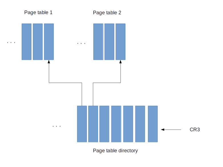
Some instructions can only be executed in ring 0. Examples are the instructions STI and CLI that start and stop interrupt processing (and potentially bring everything to a grinded halt as modern operating systems are interrupt driven, as we have seen in a previous post) or the command to reload the register CR3 which contains the base address of a page table directory and therefore the ability to load a new set of page tables. It is also possible to restrict the access to hardware using I/O ports to certain rings, so that code executing in user mode can, for instance, not directly access the hard drive or other devices.
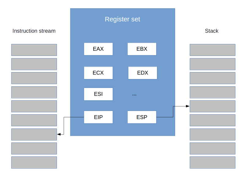
Technically, the current ring is determined by the content of a special register called the code segment register (CS) – most likely an old friend of yours if you have ever written assembly code for the 8086, we get back to this point further below. As so often in the x86 architecture, this is an indirect mechanism. The CS contains a pointer into a table called the global descriptor table (GDT) which again holds the actual descriptions of the segments. Part of each entry is a two-bit field which specifies the ring. Thus if the CS points, say, at the third entry in the GDT and those two-bits in this entry contain 0b11, the CPU executes instructions at ring 3.
Switching the privilege level
Switching the privilege level requires a bit more work than just updating CS. The easiest way to force the CPU to pick up the new settings is to raise a software interrupt (technically, there is an alternative called a far jump that we will not discuss in detail). The beauty of this is that a piece of code executing in user mode can raise an interrupt to reach ring 0, but this interrupt will execute a well defined code, namely the interrupt service handler, which again can be set up only while being in ring 0. So at startup, the operating system – executing at ring 0 – can set up the interrupt service handler to point to specific routines in the kernel, and later, during normal operations, a program executing in user mode can at any time call into the kernel by raising a software interrupt, for instance in order to read from the hard drive. However, a user mode program can only execute the specified interrupt service handler and is not able to execute arbitrary code at ring 0. Thus user mode and kernel mode are separated, but the interrupt service handlers provide specific gates to switch forth and back.
To make this work, the operating system needs to let the CPU know where each interrupt service handler is located. In protected mode, this is the purpose of the interrupt descriptor table (IDT) which an operating system needs to prepare and which contains, for each of the theoretically possible 256 interrupt service handlers, the address of the interrupt service handler as well as additional information, for instance which code segment to use (which will typically point to ring 0 to execute the interrupt in kernel mode).
My toy operating system ctOS, for instance, uses the interrupt 0x80 for system calls. A program that wants to make a system call puts a number identifying the system call into a specific register (EAX) and then raises interrupt 0x80. The interrupt service handler evaluates EAX and branches into the respective system call handler, see the ctOS system call handler documentation for more details.
Interrupts can not only be used to switch from user mode to kernel mode, but also for the way back. In fact, whenever the CPU returns from an interrupt service handler, it will return to the ring at which the execution was interrupted, using the stack to bring back the CPU into its original state. In order to move from ring 0 to ring 3, we can therefore prepare a stack that looks like being the stack arranged by the CPU if an interrupt occurs, and then execute the IRET instruction to simulate returning from an interrupt service handler.
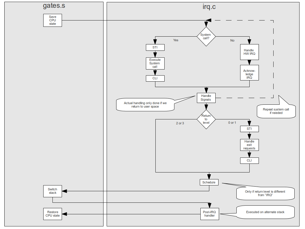
Matters get a bit more complicated by the fact that an interrupt service handler can in turn be interrupted by another interrupt, and that an operating system might want to implement kernel level threads which run outside of an interrupt context quite similar to a thread in user mode. To differentiate between those different situations, ctOS uses the concept of an execution level which is a software-maintained number describing the current context, as visualized below.

Memory model in protected mode
Another major change that the protected mode introduced into the x86 architecture was a more complex, but also more flexible memory model. To understand this, let us see how the older 8086 CPU handled memory (which is the mechanism that all modern Intel CPUs still use when being in real mode).
The 8086 was a 16-bit CPU, meaning that its registers were 16 bits wide. Therefore, a command like “put 0x10 into the memory location referenced by register AX” could only address 216=65536 different memory locations. To be able to address more memory, the Intel engineers therefore came up with a trick. When memory was accessed, the content of two registers was used. In the example above, this would be AX (16 bits) and the code segment register CS, which has 16 bits as well. To determine the actual memory location, the content of the CS register was shifted left by four bits and then added to the content of AX. Thus, if, for instance, AX contained 0x200 and CS contained 0x100, the address would be
(0x100 << 4) + 0x200 = 0x1000 + 0x200 = 0x1200
This addressing mode is sometimes called segmentation because we can think of it as dividing the memory space into (overlapping) segments of 64 kByte and the CS register as selecting one segment.
Using segmentation, the 8086 CPU could address a bit more than 1 MB of memory and thus work around the limitations of a 16 bit CPU. With a 32 bit CPU, this is not really needed any more, but the 80386 nevertheless expanded on this idea and came up with a bit more complicated model.
In fact, in protected mode, there are three different types of addresses which can be used to describe the location of a specific byte in memory.
The first type of address is the logical address. Similarly to real mode, a logical address consists of a segment selector (16 bit) which specifies the memory segment the byte is located in and an offset (32 bit) which specifies the location of the memory space within the segment.
A program running in user mode usually only sees the offset – this is what appears for instance if you dump the value of a pointer in a user mode C program. The segment selector is set by the operating system and usually not changed by a user mode program. So from the programs point of view, memory is entirely described by a 32 bit address and hence appears as a 4 GB virtual address space.
When accessing memory, the CPU uses the global descriptor table to convert this logical address into a linear address which is simply a 32 bit value. This is similar to real mode where the segment and offset are combined into a linear 20 bit wide address, with the difference that the base address of the segment is not directly taken from the CS register but the CS register only serves as pointer into the GDT that holds the actual base address.
Logical and linear address are still virtual addresses. To convert the linear address into a physical address, the CPU finally uses a page table directory and a page table as explained in one of my last posts. When the CPU has first been brought into protected mode, paging is still disabled, so this final translation step is skipped and linear and physical address are the same. Note, however, that the translation between logical and linear address cannot be turned off and is always active. So setting up this translation mechanism and in particular the GDT is one of the basis initialization step which needs to be done when switching to protected mode.

Support for hardware multi-tasking
Apart from privilege levels and virtual memory, there is even more that the protected mode can do for you. In fact, the protected mode offers hardware support for multi-tasking.
Recall from my post on multi-tasking that a task switch essentially comes down to storing the content of all registers in a safe place and restoring them later. In the approach presented in my post, this is done by manually placing the registers on a stack. However, the x86 protected mode offers an alternative – the task state segment (TSS). This is an area of memory managed by the CPU that fully describes the state of a task. An operating system can initiate a task switch, and the CPU will do all the work to reload the CPU state from the TSS.
However, this mechanism is rarely used. It has a reputation of being slower than software task switching (though I have never seen any benchmarks on this), it introduces a lot of dependencies to the CPU and I am not aware of any modern operating system using this mechanism (Linux apparently used it in early versions of the kernel). Still, at least one TSS needs to be present in protected mode even if that mechanism is not used, as the TSS is also used to store some registers when an interrupt is raised while executing in ring 3 (see the corresponding section of the ctOS documentation for more details).
Long mode
Having followed me the long and dusty road down to an understanding of the protected mode, this one will shock you: protected mode is legacy.
In fact, the protected mode as we have discussed it is a 32 bit operating mode. Since a few years, however, almost every PC you can buy is equipped with a 64 bit CPU based on the x86-64 architecture. This architecture is fully backwards compatible, i.e. you can still run a protected mode operating system on such a PC. However, this does not allow you to address more than 4 GB of memory, as pointers are limited to 32 bit.
In long mode, the CPU uses 64 bit registers and is able to use 48 bit addressing, which is good enough for 256 TB of RAM.
Fortunately, if you understand the protected mode, getting used to long mode is not too difficult. The basis concepts of the various tables that we have discussed (page tables, the IDT and the GDT) remain unchanged, but of course the layout of these tables changes to accommodate for the additional address bits. The register set, however, changes considerably. The general purpose registers are extended to 64 bits and are renamed (RAX instead of EAX etc.). In addition, a few new registers become available. There are eight additional integer registers (R8 – R15) – which are typically used to pass arguments to subroutines instead of using the stack for this purpose – and eight more SSE registers.
Apart from that, long mode is just another mode of the x86 CPU family. And this is not the end of the story – there is unreal mode, there is virtual 8086 mode, there is the system management mode and there are new modes (“VMX root mode”) that support virtualization. If you want to learn more, I recommend the excellent OSDev Wiki – maybe the most valuable single OSDev site out there – and of course the Intel Software Developer manuals. Good luck!


 and the vectors as linear combinations of tensor products to show that each hermitian operator is a linear combination of tensor products of hermitian single-qubit operators, and then use the fact that each hermitian single qubit operator is a linear combination of Pauli matrices). A tensor product of Pauli matrices corresponds to a measurement that can be easily implemented by a combination of a measurement in the standard computational basis and a unitary transformation, see for instance
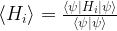
 , assuming that we can efficiently prepare the state N times and then conduct N independent measurements – in fact, if N is sufficiently large, the expectation value will simply be the average over the measurements (see
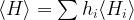
 . Let us order the eigenvalues (which are of course real) such that
  , and let us assume that
  is an orthonormal basis of corresponding eigenvectors.
 , we can of course expand this vector as a linear combination
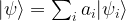
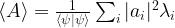

 . Thus finding an eigenvector for the lowest eigenvalue of A is equivalent to minizing the expectation value of A!
 where the parameter
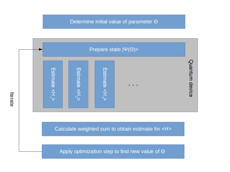
  ranges over some subset of a finite dimensional euclidian space. One then tries to minimize the expectation value
 , then determine the expectation value, adjust the parameter, determine the next expectation value and so forth. Unfortunately, calculating the expectation value of a matrix in a high dimensional Hilbert space is computationally very hard, which makes this algorithm difficult to apply to quantum systems with more than a few particles.
 where the expectation value of each
  can be efficiently determined


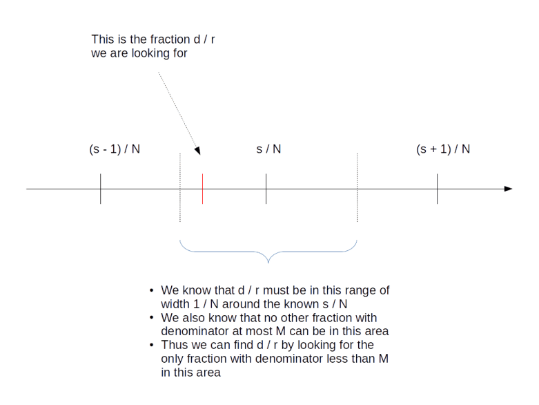
 , where N is a power of two. Getting r out of this information is again a classical step that uses the theory of continued fractions. The number N that appears here is N = 2n where n is the number of qubits that the quantum part requires, and needs to be chosen such that M2 can be represented with n bits.
 and a number
  such that gcd(x,M) = 1


 . To see how the value of the series depends on s, let us assume for a moment that the period divides N (which is very unlikely in practice as N is a power of two, but let us assume this anyway just for the sake of argument), i.e. that N = r u with the frequency u being an integer. Thus, if s is a multiple of u, the coefficient q is equal to one (as
  ) and the geometric series sums up to A, giving probability 1 / N to measure this value. If, however, s is not a multiple of u, the value of the geometric series is
 !
!
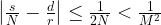
 denotes the residual of sr modulo N. Intuitively, this means that with high probability, the residual is very small, i.e. rs is close to a multiple of N, i.e. s is close to a multiple of N / r. In other words, it shows that in fact, P(s) has peaks at multiples of N / r.
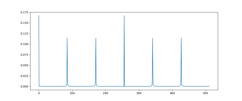


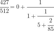
![[a_0 ; a_1, a_2, \dots ]](https://s0.wp.com/latex.php?latex=%5Ba_0+%3B+a_1%2C+a_2%2C+%5Cdots+%5D&bg=FFFFFF&fg=000&s=0&c=20201002) , we can form the continued fraction
, we can form the continued fraction
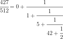
![\cfrac{427}{512} = [0; 1,5,42,2]](https://s0.wp.com/latex.php?latex=%5Ccfrac%7B427%7D%7B512%7D+%3D+%5B0%3B+1%2C5%2C42%2C2%5D++&bg=FFFFFF&fg=000&s=1&c=20201002)
![[0; 1,5,42]](https://s0.wp.com/latex.php?latex=%5B0%3B+1%2C5%2C42%5D++&bg=FFFFFF&fg=000&s=1&c=20201002)


 given by (the exact formula depends on a few conventions)


 )
) 
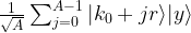
 with components
  by setting

 , this is clearly N. Otherwise, we can write this as


 due to the periodicity of the exponential function.
 . By adding a factor
  , this can be turned into a unitary transformation, i.e. in a certain sense the discrete Fourier transform is simply a rotation. This relation can also be used to easily derive a formula for the inverse of the discrete Fourier transform. In fact, if we expand the vector x into the basis
  , we obtain

 to denote the N-th root of unity, i.e.


 ! We can therefore conclude as above that this is zero unless q is one, i.e. unless k is a multiple of the frequency u. Thus we have shown that if the sequence xk is periodic with integral frequency u, then all Fourier coefficients Xk are zero for which k is not a multiple of the frequency.
  . Every vector can be described by the sequence of its coefficients when expanding it into this basis. Consequently, the discrete Fourier transform defines a unitary transformation on the Hilbert by applying the mapping


 that is zero on all but one elements. The task is to locate the element x0 for which P(x0) is true.
 of an n-qubit system to obtain a superposition of all basis states. Then, we iteratively apply the following sequence of operations.
 to
to  .
. along the diagonal, with N = 2n, and
  away from the diagonal. In terms of basis vectors, the mapping is given by

 is the average across the amplitudes
  . Thus geometrically, the operation D performs an inversion around the average. Grover shows that this operation can be written as minus a Hadamard-Walsh operation followed by the operation that flips the sign for
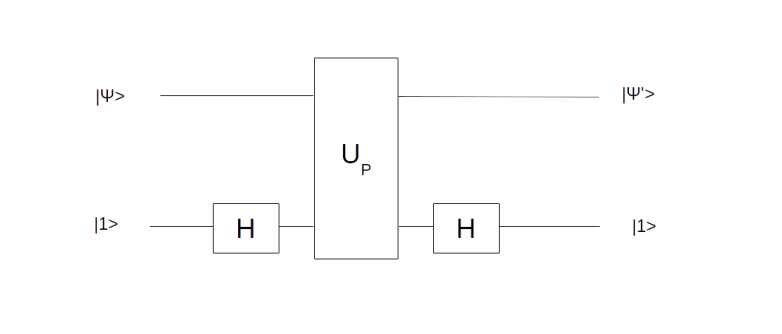

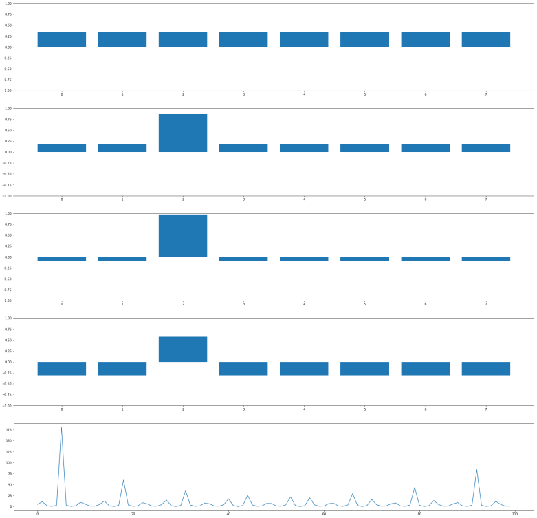
 and it will change the amplitude of this vector to – 0.35. This will change the average amplitude to a value slightly below 0.35. If we now perform the inversion around the average, the amplitudes of all basis vectors different from
  , and that doubling the number of iterations does in general lead to a less optimal result.
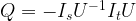
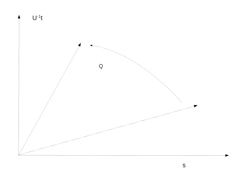
 . Applying the operation Q n times will then approximately result in a superposition of the form
 is close to a multiple of
  , then one application of U will take our state to a state very close to t.
 where x0 is the solution to the search problem. Thus the operation It is the conditional phase shift that we have denoted by S earlier. In addition, Grover shows in


 in this case, we also recover the result that the optimal number of iterations is
  applications of the transformation UP. Whether this is better than the classical algorithm does of course depend on the efficiency with which we can implement this with quantum gates. If applying UP requires O(N) operations, the advantage of the algorithm is lost. Thus the algorithm only provides a significant speedup if the operation UP can be implemented efficiently and there is no additional structure that a classical algorithm could exploit.


