Python – Page 5 – LeftAsExercise

The Metropolis-Hastings algorithm

In this post, we will investigate the Metropolis-Hastings algorithm, which is still one of the most popular algorithms in the field of Markov chain Monte Carlo methods, even though its first appearence (see [1]) happened in 1953, more than 60 years in the past. It does for instance appear on the CiSe top ten list of the most important algorithms of the 20th century (I got this and the link from this post on WordPress).

Before we get into the algorithm, let us once more state the problem that the algorithm is trying to solve. Suppose you are given a probability distribution $\pi$ on some state space X (most often this will be a real euclidian space on which you can do floating point arithmetic). You might want to imagine the state space as describing possible states of a physical system, like spin configurations in a ferromagnetic medium similar to what we looked at in my post on the Ising model. The distribution $\pi$ then describes the probability for the system to be in a specific state. You then have some quantity, given as a function f on the state space. Theoretically, this is a quantity that you can calculate for each individual state. In most applications, however, you will never be able to observe an individual state. Instead, you will observe an average, weighted by the probability of occurence. In other words, you observe the expectation value

$\langle f \rangle = \int_X f d\pi$

of the quantity f. Thus to make a prediction that can be verified or falsified by an observation, you will have to calculate integrals of this type.

Now, in practice, this can be very hard. One issue is that in order to naively calculate the integral, you would have to transverse the entire state space, which is not feasible for most realistic problems as this tends to be a very high dimensional space. Closely related to this is a second problem. Remember, for instance, that a typical distribution like the Boltzmann distribution is given by

$\pi(x) = \frac{1}{Z} e^{-\beta E(x)}$

The term in the numerator is comparatively easy to calculate. However, the term in the denominator is the partition function, and is itself an integral over the state space! This makes even the calculation of $\pi(x)$ for a single point in the state space intractable.

But there is hope – even though calculating the values of $\pi$ for one point might be impossible, in a distribution like this, calculating ratios of probabilities is easy, as the partition function cancels out and we are left with the exponential of an energy difference! The Metropolis-Hasting algorithm leverages this and also solves our state space problem by using a Markov chain to approximate the integral. So the idea is to build a Markov chain X_t that converges and has $\pi$ as an invariant distribution, so that we can approximate the integral by

$\langle f \rangle = \int_X f d\pi \approx \frac{1}{N} \sum_{t=1}^N f(X_t)$

for large values of N.

But how do we construct a Markov chain that converges to a given distribution? The Metropolis Hastings approach to solve this works as follows.

The first thing that we do is to choose a proposal density q on our state space X, i.e. a measurable function

$q \colon X \times X \rightarrow [0,\infty)$

such that for each x, $\int q(x,y) dy = 1$ .

Then q defines a Markov chain, where the probability to transition into a measurable set A being at a point x is given by the integral

$Q(x,A) = \int_{\mathcal X} q(x,y) dy$

Of course this is not yet the Markov chain that we want – it has nothing to do with $\pi$ , so there is no reason it should converge to $\pi$ . To fix this, we now adjust the kernel to incorporate the behaviour of $\pi$ . For that purpose, define

$\alpha(x,y) = \begin{cases} \min \{ 1, \frac{\pi(y)q(y,x)}{\pi(x)q(x,y)} \} & \text{if } \pi(x) q(x,y) > 0 \\ 1 & \text{if } \pi(x) q(x,y) = 0 \end{cases}$

This number is called the acceptance probability, and, as promised, it only contains ratios of probabilities, so that factors like the partition function cancel and do not have to be computed.

The Metropolis Hastings algorithm now proceeds as follows. We start with some arbitrary point x₀. When the chain has arrived at x_n, we first draw a candidate y for the next location from the proposal distribution $q(x_n, \cdot)$ . We now calculate $\alpha$ according to the formula above. We then accept the proposal with probability $\alpha$ , i.e. we draw a random sample U from a uniform distribution and accept if $U \leq \alpha$ . If the proposal is accepted, we set x_n+1 = y, otherwise we set x_n+1 = x_n, i.e. we stay where we are.

Clearly, the x_n are samples from a Markov chain, as the position at step x_n only depends on the position at step x_n-1. But is still appears to be a bit mysterious why this should work. To shed light on this, let us consider a case where the expressions above simplify a bit. So let us assume that the proposal density q is symmetric, i.e. that

$q(x,y) = q(y, x)$

This is the original Metropolis algorithm as proposed in [1]. If we also assume that $\pi$ and q are nowhere zero, the acceptance probability simplifies to

$\alpha(x,y) = \min \{ 1, \frac{\pi(y)}{\pi(x)} \}$

Thus we accept the proposal if $\pi(y) \geq \pi(x)$ with probability one. This is very similar to a random search for a global maximum – we start at some point x, choose a candidate for a point with higher value of $\pi$ at random and proceed to this point. The major difference is that we also accept candidates with $\pi(y) < \pi(x)$ with a non-zero probability. This allows the algorithm to escape a local maximum much better. Intuitively, the algorithm will still try to spend more time in regions with large values of $\pi$ , as we would expect from an attempt to sample from the distribution $\pi$ .

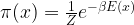
The image above illustrates this procedure. The red graph displays the distribution $\pi$ . If our algorithm is currently at step x_n, the purpose is to move “up-hill”, i.e. to the left in our example. If we draw a point like y from q which goes already in the right directory, we will always accept this proposal and move to y. If, however, we draw a point like y’, at which $\pi$ is smaller, we would accept this point with a non-zero probability. Thus if we have reached a local maximum like the one on the right hand side of the diagram, there is still a chance that we can escape from there and move towards the real maximum to the left.

In this form, the algorithm is extremely easy to implement. All we need is a function propose that creates the next proposal, and a function p that calculates the value of the probability density $\pi$ at some point. Then an implementation in Python is as follows.

import numpy as np
chain = []
X = 0
chain.append(X)
for n in range(args.steps):
  Y = propose(X)
  U = np.random.uniform()
  alpha = p(Y) / p(X)
  if (U <= alpha):
    X = Y
  chain.append(X)

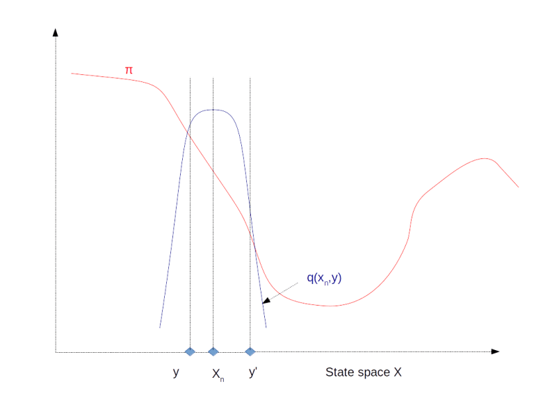
In the diagram below, this algorithm has been applied to a Cauchy distribution with mode zero and scale one, using a normal distribution with mean x and standard deviation 0.5 as a proposal for the next location. The chain was calculated for 500.000 steps. The diagram in the upper part shows the values of the chain during the simulation.

Then the first 100.000 steps were discarded and considered as "burn-in" time for the chain to stabilize. Out of the remaining 400.000 sample points, points where chosen with a distance of 500 time steps to obtain a sample which is approximately independent and identically distributed. This is called subsampling and typically not necessary for Monte Carlo integration (see [2], chapter 1 for a short discussion of the need of subsampling), but is done here for the sake of illustration. The resulting subsample is plotted as a histogramm in the lower left corner of the diagram. The yellow line is the actual probability density.

We see that after a few thousand steps, the chain converges, but continues to have spikes. However, the sampled distribution is very close to the sample generated by the Python standard method (which is to take the quotient of two independent samples from a standard normal distribution).

In the diagram at the bottom, I have displayed how the integral of two functions ( $\sin(x)$ and $\cos(x)$ ) approximated using the partial sums develops over time. We see that even though we still have huge spikes, the integral remains comparatively stable and converges already after a few thousand iterations. Even if we run the simulation only for 1000 steps, we already get close to the actual values zero (for $\sin(x)$ for symmetry reasons) and $\approx 0.3678$ (for $\cos(x)$ , obtained using the scipy.integrate.quad integration routine).

In the second diagram in the middle row, I have plotted the autocorrelation versus the lag, as an indicator for the failure of the sample points to be independent. Recall that for two samples X and Y, the Pearson correlation coefficient is the number

$\frac{E((X-\bar{X})(Y-\bar{(Y)})}{\sigma_X \sigma_Y}$

where $\sigma_X$ and $\sigma_Y$ are the standard deviations of X and Y. In our case, given a lag, i.e. a number l less than the length of the chain, we can form two samples, one consisting of the points $X_0, X_2, \dots$ and the second one consisting of the points of the shifted series $X_l, X_{l+1}, X_{l+2}, \dots$ . The autocorrelation with lag l is then defined to be the correlation coefficient between these two series. In the diagram, we can see how the autocorrelation depends on the lag. We see that for a large lag, the autocorrelation becomes small, supporting our intuition that the series and the shifted series become independent. However, if we execute several simulation runs, we will also find that in some cases, the convergence of the autocorrelation is very slow, so care needs to be taken when trying to obtain a nearly independent sample from the chain.

In practice, the autocorrelation is probably not a good measure for the convergence of a Markov chain. It is important to keep in mind that obtaining an independent sample is not the point of the Markov chain – the real point is that even though the sample is autocorrelated, we can approximate expectation values fairly well. However, I have included the autocorrelation here for the sake of illustration.

This form of proposal distributions is not the only one that is commonly used. Another choice that appears often is called an independence sampler. Here the proposal distribution is chosen to be independent of the current location x of the chain. This gives us an algorithm that resembles the importance sampling method and also shares some of the difficulties associated with it – in my notes on Markov chain Monte Carlo methods, I have included a short discussion and a few examples. These notes also contain further references and a short discussion of why and when the Markov chain underlying a Metropolis-Hastings sampler converges.

Other variants of the algorithm work by updating – in a high-dimensional space – either only one variable at a time or entire blocks of variables that are known to be independent.

Finally, if we are dealing with a state space that can be split as a product $X_1 \times X_2$ , we can use the conditional probability given either x₁ or x₂ as a proposal distribution. Thus, we first fix x₂, and draw a new value for x₁ from the conditional probability for x₁ given the current value of x₂. Then we move to this new coordinate, fix x₁, draw from the conditional distribution of x₂ given x₁ and set the new value of x₂ accordingly. It can be shown (see for example [5]) that the acceptance probability is one in this case. So we end up with the Gibbs sampling algorithm that we have already used in the previous post on Ising models.

Monte Carlo sampling methods are a broad field, and even though this has already been a long post, we have only scratched the surface. I invite you to consult some of the references below and / or my notes for more details. As always, you will also find the sample code on GitHub and might want to play with this to reproduce the examples above and see how different settings impact the result.

In a certain sense, this post is the last post in the series on restricted Boltzmann machines, as it provides (at least some of) the mathematical background behind the Gibbs sampling approach that we used there. Boltzmann machines are examples for stochastic neuronal networks that can be applied to unsupervised learning, i.e. the allow a model to learn from a sample distribution without the need for labeled data. In the next few posts on machine learning, I will take a closer look at some other algorithms that can be used for unsupervised learning.

References

1. N. Metropolis,A.W. Rosenbluth, M.N. Rosenbluth, A.H. Teller, E. Teller, Equation of state calculation by fast computing machines, J. Chem. Phys. Vol. 21, No. 6 (1953), pp. 1087-1092
2. S. Brooks, A. Gelman, C.L. Jones,X.L. Meng (ed.), Handbook of Markov chain Monte Carlo, Chapman Hall / CRC Press, Boca Raton 2011
3. W.K. Hastings, Monte Carlo sampling methods using Markov chains and their applications, Biometrika, Vol. 57 No. 1 (1970), pp. 97-109
R.M. Neal, Probabilistic inference using Markov chain Monte Carlo methods, Technical Report CRG-TR-93-1, Department of Computer Science, University of Toronto, 1993
5. C.P. Robert, G. Casella, Monte Carlo Statistical Methods,
Springer, New York 1999

The difficulty in the bitcoin protocol

Mining is a challenge – a miner has to solve a mathematical puzzle to create a valid block and is rewarded with a certain bitcoin amount (12.5 at the time of writing) for investing electricity and computing power. But technology evolves, and the whole mining process would be pointless if the challenge could not be adapted dynamically to make sure that mining power and the difficulty of the challenge stay in balance. In this post, we will look in a bit more detail into this mechanism.

We have already seen that a block header contains – at character 144 – a four byte long number that is called bits in the source code and which seems to be related to the difficulty. As an example, let us take the block with the hash

0000000000000000000595a828f927ec02763d9d24220e9767fe723b4876b91e

You can get a human readable description of the block at this URL and will see the following output.

This output has a field bits that has the value 391129783. If you convert this into a hexadecimal string, you obtain 0x17502ab7, using for instance Pythons hex function. Now this function will give you the big-endian representation of the integer value. To convert to little endian as it can be found in the serialized format of a bitcoin block, you have to reverse the order byte wise and get b72a5017. If you now display the raw format of the block using this link and search for that string, you will actually find it at character 144 at expected.

Now on the screenshot above, you also see the difficulty displayed, which is a floating point number and is 3511060552899.72 in this case. How is that difficulty related to the bits?

As so often, we can find the answer in the bitcoin core source code, starting at the JSON RPC interface. So let us look at the function blockheaderToJSON in rpc/blockchain.cpp that is responsible for transforming a block in the internal representation into a human readable JSON format. Here we find the line

result.push_back(Pair("difficulty", GetDifficulty(blockindex)));

So let us visit the function GetDifficulty that we find in the same file, actually just a few lines up. Here we see that the bits are actually split into two parts. The first part, let me call this the size is just the value of the top 8 bits. The second part, the value of remaining 24 bits, is called the coefficient. Then the difficulty is calculated by dividing the constant 0xFFFF by the coefficient and shifting by 29 – size bits, i.e. according to the formula

$\text{difficulty} = 256^{(29 - \text{exponent})} \cdot (65535.0 / \text{coefficient})$

In Python, we can therefore use the following two lines to extract the difficulty from a block header in raw format.

nBits = int.from_bytes(bytes.fromhex(raw[144:152]), "little")
difficulty = 256**(29 - (nBits >> 24))*(65535.0 / ((float)(nBits & 0xFFFFFF)))

If you try this out for the transaction above, you will get 3511060552899.7197. Up to rounding after the second digit after the decimal point, this is exactly what we also see on the screenshot of blockchain.info. So far this is quite nice…

However, we are not yet done – this is not the only way to represent the difficulty. The second quantity we need to understand is the target. Recall that the mathematical puzzle that a miner needs to solve is to produce a block with a hash that does not exceed a given number. This number is the target. The lower the target, the smaller the range of 256 bit numbers that do not exceed the target, and the more difficult to solve that puzzle. So a low target implies high difficulty and vice versa.

In fact, there are two target values. One target is part of every block and stored in the bits field – we will see in a minute how this works. The second target is a global target that all nodes in the bitcoin network share – this value is updated independently by each node, but based on the same data (the blockchain) and the same rules so that they arrive at the same conclusion. A block considered valid if solves the mathematical puzzle according to the target which is stored in itself and if, in addition, this target matches the global target.

To understand how this works and the exact relation between target and difficulty, it is again useful to take a look at the source code. The relevant function is the function CheckProofOfWork in pow.cpp which is surprisingly short.

bool CheckProofOfWork(uint256 hash, unsigned int nBits, const Consensus::Params& params)
{
    bool fNegative;
    bool fOverflow;
    arith_uint256 bnTarget;

    bnTarget.SetCompact(nBits, &fNegative, &fOverflow);

    // Check range
    if (fNegative || bnTarget == 0 || fOverflow || bnTarget > UintToArith256(params.powLimit))
        return false;

    // Check proof of work matches claimed amount
    if (UintToArith256(hash) > bnTarget)
        return false;

    return true;
}

Let us try to understand what is going on here. First, a new 256 bit integer bnTarget is instantiated and populated from the bits (that are taken from the block) using the method SetCompact. In addition to a range check, it is then checked that the hash of the block does not exceed the target – this the mathematical puzzle that we need to solve.

The second check – verifying that the target in the block matches the global target – happens in validation.cpp in the function ContextualCheckBlockHeader. At this point, the function GetNextWorkRequired required is called which determines the correct value for the global target. Then this is compared to the bits field in the block and the validation fails if they do not match. So for a block to be accepted as valid, the miner needs to:

Actually solve the puzzle, i.e. provide a block with a hash value equal to or smaller than the current global target
Include this target as bits in the generated block

This leaves a couple of questions open. First, we still have to understand how the second step – encoding the target in the bits field – works. And then we have to understand how the global target is determined.

Let us start with the first question. We have seen that the target is determined from the bits using the SetCompact method of the class uint256. This function is in fact quite similar to GetDifficulty studied before. Ignoring overflows and signs for a moment, we find that the target is determined from the bits as

$\text{target} = \text{coefficient}\cdot 2^{8(\text{exponent}-3)}$

If we compare this to the formula for the difficulty that we have obtained earlier, we find that there a simple relation between them:

$\text{target} = \text{difficulty}^{-1}\cdot \text{std\_target}$

where std_target is the target corresponding to difficulty 1.0 and given by 0xFFFF shifted by 208 bits to the left, i.e. by 0xFFFF with 52 trailing zeros. So up to a constant, target and difficulty are simply inverse to each other.

Now let us turn to the second question – how can the nodes agree on the correct global target? To see this, we need to look at the function GetNextWorkRequired. In most cases, this function will simply return the bits field of the current last block in the blockchain. However, every 2016 blocks, it will adjust the difficulty according to the following rule.

First, it will use the time stamps in the block to calculate how much time has passed since the block which is 2016 blocks back in the chain has been created – this value is called the actual time span. Then, this is compared with the target time span which is two weeks. The new target is then obtained by the formula (ignoring some range checks that are done to avoid too massive jumps)

$\text{target}_{new} = \text{target}_{old} \cdot \frac{\text{actual time span}}{\text{target time span}}$

Thus if the actual time span is smaller than the target time span, indicating that the mining power is too high and therefore the rate of block creation is too high, the target decreases and consequently the difficulty increases. This should make it more difficult for the miners to create new blocks and the block creation rate should go down again. Similarly, if the difficulty is too high, this mechanism will make sure that it is adjusted downwards. Thus the target rate is 2016 blocks being created in two weeks, i.e. 336 hours, which is a rate of six blocks per hours, i.e. 10 minutes for one block.

Finally, it is worth mentioning that there is lower limit for the difficulty, corresponding to a higher limit for the target. This limit is (as most of the other parameters that we have discussed) contained in chainparams.cpp and specific for the three networks main, net and regtest. For instance, for the main network, this is

consensus.powLimit = uint256S("00000000ffffffffffffffffffffffffffffffffffffffffffffffffffffffff");

whereas the same parameter for the regression testing network is

consensus.powLimit = uint256S("7fffffffffffffffffffffffffffffffffffffffffffffffffffffffffffffff");

This, together with the target of the genesis block (which determines the target for the first 2016 blocks) (bits = 0x207fffff ) determines the initial difficulty in a regression test network. Let us verify this (I knew I would somehow find a reason to add a notebook to this post…)

Sorry, something went wrong. Reload?

Sorry, we cannot display this file.

Sorry, this file is invalid so it cannot be displayed.

view raw InitialDifficultyRegTest.ipynb hosted with ❤ by GitHub

We are now well equipped to move towards our final project in this series – building a Python based miner. The last thing that we need to understand is how the miner operates and communicates with the bitcoin server, and this will be the topic of the next post.

Recurrent and ergodic Markov chains

Today, we will look in more detail into convergence of Markov chains – what does it actually mean and how can we tell, given the transition matrix of a Markov chain on a finite state space, whether it actually converges.

So suppose that we are given a Markov chain on a finite state space, with transition probabilities described by a matrix K as in the previous post on this topic.

We have seen that the distribution of X_n is given by $\mu K^n$ where $\mu$ is the initial distribution. So if Kⁿ converges, we can expect the distribution of X_n to converge as well. If there is a matrix $K^\infty$ such that

$\lim_{n \rightarrow \infty} K^n = K^\infty$

then of course

$K^\infty K = (\lim_{n \rightarrow \infty} K^n) K = \lim_{n \rightarrow \infty} K^{n+1} = K^\infty$

In other words, each row $\pi$ of $K^\infty$ will have the property that $\pi K = \pi$ . Interpreting K as transition probabilities, this implies that if the distribution of X_n is $\pi$ , the distribution of X_n+1 will again be $\pi$ . Any distribution, described by a row vector $\pi$ with row sum 1, for which this holds is called an invariant distribution and traditionally denoted by $\pi$ . In other words, invariant distributions correspond to eigenvectors of the transposed matrix K^T with eigenvalue 1, and our argument has shown that if $K^n$ converges to $K^\infty$ , then every row of $K^\infty$ will be an invariant distribution.

So convergence implies the existence of an invariant distribution. Let us next try to understand whether this invariant distribution is unique. There are obvious examples where this is not the case, the most trivial one being the unit matrix

$K = \begin{pmatrix} 1 & 0 \\ 0 & 1 \end{pmatrix}$

Obviously $K^n = K$ and the chain converges, but every vector with row sum one is an invariant distribution. This chain is too rigid, because in whatever state we start, we will stay in this state forever. It turns out that in order to ensure uniquess of an invariant distribution, we need a certain property that makes sure that the states can move around freely which is called irreducibility.

Intuitively, we say that a Markov chain is irreducible if any state can be reached from any other state in finitely many steps. For a finite state space, this is rather easy to formalize. A finite Markov chain is called irreducible if, given two states i and j, we can find some power n such that $K^n_{ij} > 0$ . In other words, given a row index i and a column index j, we can find a power n such that the element of Kⁿ at (i,j) is not zero. It turns out that if a chain is not irreducible, we can split the state space into smaller areas that the chain – once it has entered one of them – does not leave again and on which it is irreducible. So irreducible Markov chains are the buildings blocks of more general Markov chains, and the study of many properties of Markov chains can be reduced to the irreducible case.

Now let us assume that our chain is in fact irreducible. What else do we have to ask for to make sure that it converges? Again, let us as look at an obvious example.

$K = \begin{pmatrix} 0 & 1 \\ 1 & 0 \end{pmatrix}$

All even powers of this matrix are the unit matrix and all odd powers are K itself, so the Markov chain described by this transition matrix is clearly irreducible. However, there is still something wrong. If, for instance, we are in state 1 at the time t, then the probability to still be in state 1 at time t+1 is zero. Thus we are actually forced to move to state 2. In a certain sense, there is still an additional constraint on the the behaviour of the chain – the state space can be split in two pieces and we cycle through these pieces with every step. Such a chain is called periodic. If a chain is periodic, it is again obvious that we can think of it as two different chains, one chain given by the random variables X₀, X₂,… at even times and the other chain given by the random variables X₁, X₃, … at odd times. Thus again, there is a way to split the chain into parts.

So let us now focus on chains that are irreducible and aperiodic. Can we tell whether the chain converges? The answer is surprisingly simple and one of the most powerful results in the theory or Markov chains: every finite Markov chain which is irreducible and aperiodic converges. Thus once we have verified aperiodicity and irreducibility, we can be sure that the limit $K^\infty$ exists. We can say even more – we have seen that the rows of the limit are invariant distributions for K. However, one can show that an irreducible Markov chain can only have one invariant distribution. Thus we can conclude that all rows of the matrix $K^\infty$ are identical. In fact, they are all equal to the (unique) invariant distribution that again corresponds to an eigenvector of K^T with eigenvalue one.

This gives us two different approaches to calculating the invariant distribution and the limit $K^\infty$ . First, we can form high powers Kⁿ to approximate the limit $K^\infty$ . Or, alternatively, we can search for eigenvectors of the transposed matrix K^T with eigenvalue 1 using one of the known algorithms to calculate eigenvectors and eigenvalues.

Let us do this for the example of the random walk on a circle that we have studied earlier. For simplicity, we will use N = 4 this time. The transition matrix with p = 0.8 is

$K = \begin{pmatrix} 0.20 & 0.40 & 0.00 & 0.40 \\ 0.40 & 0.20 & 0.40 & 0.00 \\ 0.00 & 0.40 & 0.20 & 0.40 \\ 0.40 & 0.00 & 0.40 & 0.20 \\ \end{pmatrix}$

We can then easily implement both approaches in Python using the numpy library.

Sorry, something went wrong. Reload?

Sorry, we cannot display this file.

Sorry, this file is invalid so it cannot be displayed.

view raw TransitionMatrixMarkovChain.ipynb hosted with ❤ by GitHub

So we see that the approach to take the eigenvalues and eigenvectors gives us – in this case – the exact result (and a direct computation confirms that this is really an eigenvector), whereas the matrix power with n=20 gives a decent approximation. Both results confirm what we have observed visually in the last post – the distribution converges, and it does in fact converge to the uniform distribution. So roughly speaking, after sufficiently many steps, we end up everyhwere in the state space with equal probability.

So far, we have only discussed the case of a finite state space. In the general case, the situation is more complicated. First, we need a better definition of irreducibility, as on a general state space, the probability measure of a single point tends to be zero. It turns out that the solution is to define irreducibility with respect to a measure on the state space, which is called $\psi$ -irreducibility. Once we have that, we find two potential behaviours that do not show up in the finite case.

First, it might happen that even though the chain is irreducible, it does not properly cycle through the state space and revisits every point with finite probability, but – intuitively speaking – heads off to infinity. Such a chain is called transient and does not converge.

Second, even if the chain is not transient, we might be able to find an invariant distribution (a measure in this case), but this measure might not be a probability distribution as it is not finite. Chains with this property are called null recurrent.

And finally, the concept of converge needs to be made more precise, and it turns out to have a subtle dependency on the starting point which can be fixed by assuming so called Harris recurrence. But all this can be done and delivers a very similar result – a convergence theorem for a large class of chains (in this case aperiodic Harris recurrent Markov chains). If you would like to get deeper into this and also see proofs for the claims made in this post and references, I invite you to take a look at my short introduction to Markov chains.

We close this post with one remark which, however, is of crucial importance for applications. Suppose we have a convergent Markov chain X_t, and a function f on the state space. If the X_t were independent and identically distributed, we could approximate the expectation value of f as

$\int_X f(x) dP = \lim_{N \rightarrow \infty} \frac{1}{N} \sum_{i=1}^N f(X_i)$

where dP is the (common) distribution of the X_t. For Markov chains, however, we know that the X_t are not independent – the whole point of having a Markov chain is that X_t+1 does actually depend on X_t. However, in our example above, we have seen that the dependency gets trivial for large t as in this example, all entries in the transition matrix become equal in the limit.

Of course this is a special case, but it turns out that even in general, the approximation of the expectation value by averages across the sample is still possible. Intuitively, this is not so surprising at all. If the distributions $K^n$ of the $X_n$ converge to some invariant measure $\pi$ , the $X_n$ will, for large n, be approximately identically distributed, namely according to $\pi$ . Moreover, heuristically we have for large n, m and a fixed starting point s:

$P(X_{n+m}=i, X_n=j) = K^m_{ji} K^n_{sj} \approx \pi_i \pi_j$

On the other hand, this product is again approximately the product

$\pi_i \pi_j \approx P(X_{n+m}=i) P(X_n=j)$

Thus, intuitively, X_n and X_m are almost independent if n and m are large, which makes us optimistic that the law of large numbers could actually hold.

In fact, if X_t converges (again I refer to my notes for a more precise definition of convergence in this case), it turns out that the law of large numbers remains valid if we integrate f with respect to the invariant distribution $\pi$ :

$\int_X f(x) d\pi = \lim_{N \rightarrow \infty} \frac{1}{N} \sum_{i=1}^N f(X_i)$

This is extremely useful in applications, where often the primary purpose is not so much to obtain a sample, but to approximate otherwise intractable integrals! Once we have found a Markov chain that converges to the invariant distribution $\pi$ , we can calculate integrals over $\pi$ by running a long Markov chain until converge and then taking the average value of the function that we want to integrate for a large number of subsequent points from this chain. In fact, this is how most applications work – and this is more or less what we also did when we applied Markov chains to the problem of calculating gradients in the PCD algorithm, where this chain is given by the state of the negative particles in subsequent iterations.

So given a distribution $\pi$ , we are now lead to the question how we can possibly find a Markov chain for which this distribution is invariant and which converges. The most general answer to this question is a class of algorithms known as Metropolis-Hastings algorithms which we study in the next post in this series.

Merkle trees

Suppose you are given a long file and wanted to use hashing to verify the integrity of the file. How would you do this in the most efficient way?

Of course, the first thing that might come to your mind is to simply take a hash of the entire file. This is very easy, but has one major disadvantage – if the file is damaged, there is no way to tell which part of the file has been damaged. If you use such a mechanism for instance to verify the integrity of a large download, you will have to go back and download the entire file again, which is very time consuming.

A smarter approach is to split the file into data blocks. You then calculate a hash for each data block to obtain a hash list. Finally, you could concatenate all the hashes into one large string and take the hash of that string. If a recipient of the file has access to only this top level hash, she could already verify the integrity of the file by repeating this procedure and comparing the top level hash with the hash created by the sender.

If that check fails, there is no need to re-transmit the entire file. Instead, the recipient could obtain a copy of the hash list itself and compare the hashes block by block until the faulty block is detected. This block can then be exchanged and the procedure can be repeated to verify that the replacement is valid. The bittorrent protocol uses this mechanism to detect inconsistencies in transferred files.

With a simple hash list like this, you would have to search the entire hash list in order to determine the faulty piece, requiring a time linear in the number of blocks. Searching can be improved greatly by organizing the hashes not into a list, but into a (binary) tree – and this data structure is called a hash tree or Merkle tree.

To illustrate the principle, suppose you wanted to build a hash tree for a file consisting of eight blocks, labeled 1 – 8.

You would then proceed as follows, as indicated in the image above. First, you compute the hash value for all blocks and assign them as values to the eight leaves of the tree. Then, you concatenate the values of leaves 1 and 2 and take the hash value of the result. This gives you the value for the parent node – called a in the picture above – of 1 and 2. You repeat the same procedure for the leaves 3 and 4, this gives you the value for the node b. Then you concatenate the values of a and b and take the hash value of the result, this gives you the value of the node c. Repeat this procedure for the right part of the tree and assign the result to node d. Finally, concatenate the values of node c and d and take the hash – this will be the value of the root node called the Merkle root. Thus, in a binary Merkle tree, the value of each node is defined to be the hash of the concatenation of the values of its two child nodes.

How is a Merkle tree realised in the bitcoin reference implementation? The currently relevant code is in consensus/merkle.cpp. This implementation is already optimized, the original implementation used to be in primitives/block.cpp and is still available on GitHub.

As the comments in the source code explain, at any level of the tree, the last node is added at the end again if needed to make sure that the number of nodes is even at each level – the algorithm that I have illustrated above only works if the number of leaves is a power of two. The actual implementation first builds a list of the leaves. It then goes through the list and for any two subsequent elements, it adds an element at the end which is the hash of the concatenation of these two elements. The last element is then the Merkle root that we are looking for.

Let us now see how a straightforward implementation looks like in Python.

Sorry, something went wrong. Reload?

Sorry, we cannot display this file.

Sorry, this file is invalid so it cannot be displayed.

view raw MerkleRoot.ipynb hosted with ❤ by GitHub

Most of the code should be self explaining, but a few remarks are in order. First, the hash function that we use could of course by any hash function, but, to be consistent with what bitcoin is doing, we use a double SHA256 hash. Then, byte ordering is again to be observed. The bitcoin reference client uses the method GetHash() on the involved transactions to populate the leaves, and we know that this is providing the transaction ID in little endian byte order. The entire calculation then proceeds in little endian byte order. The JSON output, however, display the transaction IDs in big endian order and the same holds for the Merkle root. Thus we need to reverse the byte order before we build the tree and, when comparing our result with the Merkle root which is part of the block, reverse the byte order again.

The actual calculation of the Merkle root uses a very straightforward approach – instead of maintaining one long list as the original bitcoin reference representation did, we represent the nodes at each level of the tree by a separate list and use recursion. This is probably a bit less efficient, but maybe easier to understand.

In order to test our implementation, we finally use the Python requests library to get a block in JSON format from blockchain.info using their REST API. We then build the leaves of the tree by walking through the list of transaction IDs in the block, build the Merkle root and compare the result to the value which is part of the JSON block structure. Nice to see that they match!

What happens if a client wants to verify that a given transaction is really included in a block without downloading the full block? In this case, it can ask the bitcoin server (either via the RPC call gettxoutproof or as part of the GETDATA network message) to provide a Merkle block, which is a serialized instance of CMerkleBlock. Essentially, a Merkle block consists of a block header plus a branch of the Merkle tree that is required to verify that a specific transaction is part of the block. This eliminates the need to transfer all transactions (which can be several thousand) while still allowing the client to check that a transaction is really included in a block.

This completes our short discussion of Merkle trees. We are now able to calculate the Merkle root for inclusion in a block header given the list of transactions that a block contains. To be able to mine a block, there is one more thing that we need to understand and that we will cover in the next post in this series – mining difficulty and the proof-of-work target.

Finite Markov chains

In this post, we will look in more detail into an important class of Markov chains – Markov chains on finite state spaces. Many of the subtleties that are present when studying Markov chains in general state spaces do not appear in the finite case, while most of the key ideas and features of Markov chains are still visible, so this is a good starting point if you want to grasp the key points.

So let us assume that our state space X is finite. For simplicity, we label our states as $\{1, 2, \cdots N \}$ where N is the number of states. We also assume that all our points are measurable, i.e we consider our state space as a discrete probability space.

Now consider a sequence of random variables X₀, X₁, …. How can we formalize the idea that X_t+1 depends on X_t in a randomized way?

As so often in probability theory, let us model the dependency as a conditional probability. The conditional probability for X_t+1 to take on a value i given X_t

$P(X_{t+1} = i | X_t)$

considered as a function of X_t will assign a conditional probability to each of the states i and for each value of X_t. Therefore we can write this as a matrix

$P(X_{t+1} = i | X_t = j) = K_{ji}$

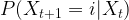
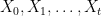
To obtain a time homogeneous Markov chain, we also assume that the matrix K does not depend on the time t. Therefore we define a Markov chain on X to be a sequence $\{X_t\}_t$ of random variables taking values in X with the Markov property saying that for all times t, the conditional distribution for X_t+1 given all previous values $X_0, X_1, \dots, X_t$ only depends on X_t, i.e.

$P(X_{t+1} | X_t, X_{t-1}, \cdots ) = P(X_{t+1} | X_t)$

We also require that this conditional probability is independent of t and is therefore given by a matrix K as in the formula above.

Markov chains on finite state spaces are often visualized as a graph. Suppose, for instance, that our state space contains only two elements: $X = \{ 1 , 2\}$ . We can think of the combined values $X_t$ for all times t as a history of states or as a random walk in the state space. The Markov property then means that the probability to transition into a next state does not depend on the full history, but only on the current state – Markov chains do not have a memory.

In our state space with two elements only, the Markov chain is then described by four transition probabilities: the probability to stay in state 1 when the chain is in state 1, the probability to move to state 2 when being in state 1, the probability to stay in state 2 and the probability to move to state 1 after being in state 2. This can be visualized as follows.

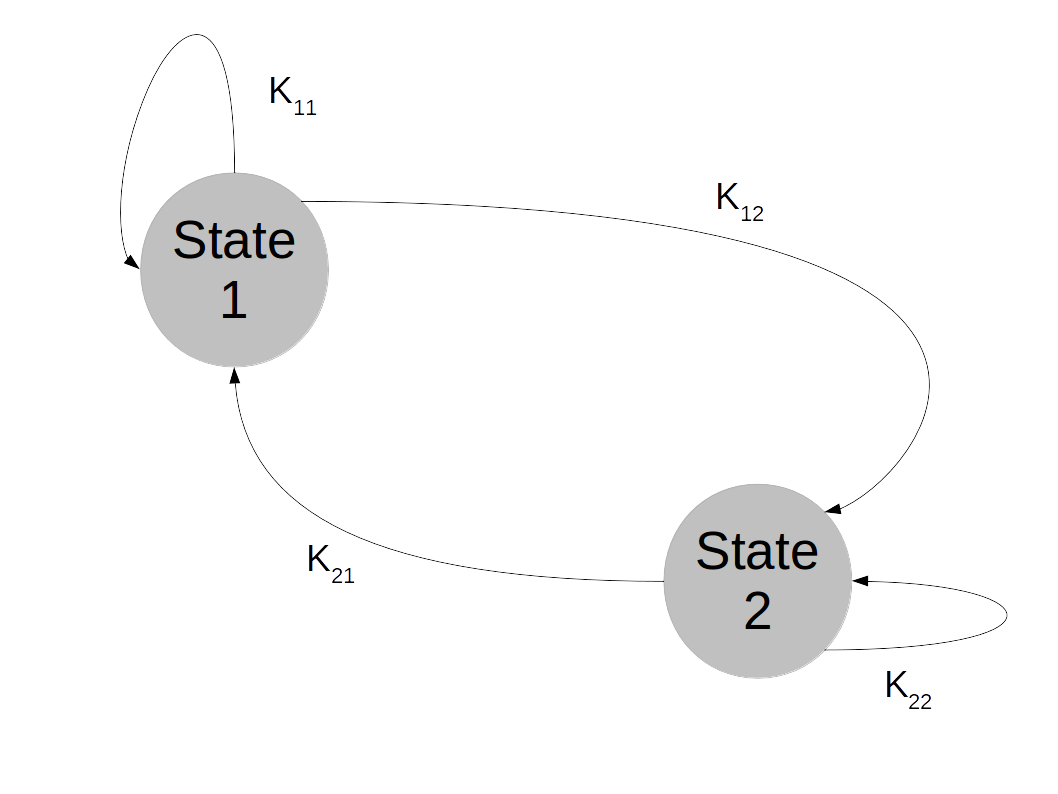
Let us now calculate a few probabilities to get an idea for the relevant quantities in such a model. First, suppose that at time 0, the model is in state j with probability $\mu_j$ . What is the probability to be in state j after one step? Of course we can write

$P(X_1 = i) = \sum_j P(X_1 = i, X_0 = j)$

Now, according to the rules of conditional probabilities, we can express the joint probability as follows.

$P(X_1 = i, X_0 = j) = P(X_1 = i | X_0 = j) P(X_0 = j)$

Plugging this into our previous expression and using the definitions of K and $\pi$ , we now obtain

$P(X_1 = i) = \sum_j K_{ji} \mu_j$

Thus if we think of $\mu$ as a row vector, then the probability after one step is described by the matrix product $\mu K$ .

Now let us calculate a slightly different quantity. Assume that we know that a chain starts at j. What is the probability to be at i after two steps? Using once more the rules of conditional probability and the Markov property, we can write

$P(X_2=i | X_0=j) = \sum_k P(X_2=i | X_1=k)P(X_1=k | X_0=j)$

Intuitively, this is very appealing. To get from j to i in two steps, we can take the way via any intermediate state k. To get the total probability, we simply sum up all these different probabilities! If you have ever seen path integrals in quantum mechanics, this idea will look familiar.

Again, we can write this in matrix notation. Each of the conditional probabilities on the right hand side of the expression above is a matrix element, and we find that

$P(X_2 = i | X_0 = j) = \sum_k K_{ki} K_{jk}$

so that the probability to get in two steps from j to i is simply given by the elements of the matrix K². Similarly, the n-step transition probabilities are the entries of the matrix Kⁿ.

Let us look at an example to understand what is going on here, which is known as a finite random walk on a circle. Our state space consists of N distinct points which we place arbitrarily on a circle. We then define a Markov chain as follows. We start at some arbitrary point x. In each step, we move along the circle to a neighbored point – one point to the left with probability 1/2 and one point to the right with probability 1/2. By the very definition, the transition probabilities do not change over time and depend only on the current state, so is a finite Markov chain. 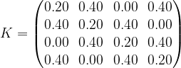If we label the points on the circle by $1, 2, \dots, N$ , then the transition matrix is given by a matrix of the form (for instance for N=4)

$K = \begin{pmatrix} 0 & \frac{1}{2} & 0 & \frac{1}{2} \\ \frac{1}{2} & 0 & \frac{1}{2} & 0 \\ 0 & \frac{1}{2} & 0 & \frac{1}{2} \\ \frac{1}{2} & 0 & \frac{1}{2} & 0 \end{pmatrix}$

More generally, we can also allow the process to stay where it is with probability 1 – p, where p is then the probability to move, which leads us to the matrix

$K = \begin{pmatrix} 1-p & \frac{p}{2} & 0 & \frac{p}{2} \\ \frac{p}{2} & 1-p & \frac{p}{2} & 0 \\ 0 & \frac{p}{2} & 1-p & \frac{p}{2} \\ \frac{p}{2} & 0 & \frac{p}{2} & 1 - p \end{pmatrix}$

Let us try to figure out whether the target distribution, given by the matrix Kⁿ for large n, somehow converges.

To see this, we do two numerical experiments. First, we can easily simulate a random walk. Suppose that we have a function draw which accepts a distribution (given by a vector p whose elements add up to one) and draws a random value according to that distribution, i.e. it returns 1 with probability p₀, 2 with probability p₁ and so on. We can then simulate a random walk on the circle as follows.

def simulate_chain(N, p, steps=100, start=5):
    chain = []
    x = start % N
    chain.append(x)
    for i in range(steps):
        x = (x  + draw([p/2.0, 1.0 - p, p / 2.0]) - 2) % N
        chain.append(x)
    return chain

Here N is the number of points on the circle, steps is the number of simulation steps that we run and start is the starting point. The function draw then returns 1 with probability p/2, 3 with probability p/2 and 2 with probability 1 – p. Thus we move with probability p/2 to the right, with probability p/2 to the left and stay were we are with probability 1 – p. If we set p = 0.8, this results in the following transition matrix.

$\begin{pmatrix} 0.20 & 0.40 & 0.00 & 0.00 & 0.00 & 0.00 & 0.00 & 0.00 & 0.00 & 0.40 \\ 0.40 & 0.20 & 0.40 & 0.00 & 0.00 & 0.00 & 0.00 & 0.00 & 0.00 & 0.00 \\ 0.00 & 0.40 & 0.20 & 0.40 & 0.00 & 0.00 & 0.00 & 0.00 & 0.00 & 0.00 \\ 0.00 & 0.00 & 0.40 & 0.20 & 0.40 & 0.00 & 0.00 & 0.00 & 0.00 & 0.00 \\ 0.00 & 0.00 & 0.00 & 0.40 & 0.20 & 0.40 & 0.00 & 0.00 & 0.00 & 0.00 \\ 0.00 & 0.00 & 0.00 & 0.00 & 0.40 & 0.20 & 0.40 & 0.00 & 0.00 & 0.00 \\ 0.00 & 0.00 & 0.00 & 0.00 & 0.00 & 0.40 & 0.20 & 0.40 & 0.00 & 0.00 \\ 0.00 & 0.00 & 0.00 & 0.00 & 0.00 & 0.00 & 0.40 & 0.20 & 0.40 & 0.00 \\ 0.00 & 0.00 & 0.00 & 0.00 & 0.00 & 0.00 & 0.00 & 0.40 & 0.20 & 0.40 \\ 0.40 & 0.00 & 0.00 & 0.00 & 0.00 & 0.00 & 0.00 & 0.00 & 0.40 & 0.20 \\ \end{pmatrix}$

We can visualize the results if we execute a large number of runs and draw histograms of the resulting positions 100, 200, 300, … steps. The result will look roughly like this (for this image, I have used p = 0.8 and N=10):

We see that after a few hundred steps, this seems to converge – actually this starts to look very much like a uniform distribution. As we already know that the distribution after n steps is given by the matrix Kⁿ, it makes sense to look at high powers of this matrix as well. To visualize this, I will use a method that I have seen in MacKays excellent book and that works as follows.

Visualizing one row of a matrix is not difficult. We can plot the entries in a two-dimensional diagram, where the x-axis corresponds to the column index and the y-axis corresponds to the value. A flat line is then a row in which all entries have the same value.

To display a full matrix, we use colors – we assign one color to each row index and plot the individual rows as just described. If we do this for the powers of the matrix K with the parameters p = 0.8 and N = 10 (and only chose some rows, for instance 1,4,7, to not run out of colors…) we obtain an image like the one below.

We can clearly see that the powers of the matrix K converge towards a matrix

$K^\infty = \lim_{n \rightarrow \infty} K^n$

where all entries in each row seem to have the same value. We have seen that the distribution after n steps assuming an initial distribution described by a row vector $\mu$ is $\mu K^n$ . Therefore the limit distribution is $\mu K^\infty$ . If we take $\mu$ to be a unit vector, we find that the rows of the matrix $K^\infty$ do actually represent the limit distribution of all chains that have started at a specific point i of the state space. Therefore the entries in the rows need to sum up to one, and thus, if they are all equal, need to be equal to 1 / N. If you calculate and print out high powers of the matrix K, you will in fact see that they approach the matrix where all entries are 0.1 (as we have chosen N = 10 in this example).

To completes our short introduction into Markov chains. We have seen that Markov chains model stochastic processes in discrete time in which the state at step t+1 depends only on the state at step t and the dependency is given by a function independent of the current time. In finite state spaces, Markov chains are described by a transition matrix K. The i-th row of the matrix Kⁿ is the distribution of chains starting at point i after n steps. Consequently, converge properties of the Markov chains can be related to converge of high powers Kⁿ and the apparatus of linear algebra can be applied.

In the next post, we will learn more about convergence – how it can be made precise, and how we can tell whether a given Markov chain converges. This will then allow us to construct Markov chains that converge towards a given target distribution and use them for sampling.

Understanding bitcoin blocks

In order to analyse a block, obviously the first thing that we need is – a block. Fortunately, this is not difficult. We can either use the block explorer hosted by blockchain.info to get the second block in the blockchain in raw or JSON or use curl to retrieve the block from the command line, say in raw format.

$ curl https://blockchain.info/de/block/000000006a625f06636b8bb6ac7b960a8d03705d1ace08b1a19da3fdcc99ddbd?format=hex

010000004860eb18bf1b1620e37e9490fc8a427514416f
d75159ab86688e9a8300000000d5fdcc541e25de1c7a5a
ddedf24858b8bb665c9f36ef744ee42c316022c90f9bb0
bc6649ffff001d08d2bd61010100000001000000000000
0000000000000000000000000000000000000000000000
000000ffffffff0704ffff001d010bffffffff0100f205
2a010000004341047211a824f55b505228e4c3d5194c1f
cfaa15a456abdf37f9b9d97a4040afc073dee6c8906498
4f03385237d92167c13e236446b417ab79a0fcae412ae3
316b77ac00000000

For this post, I have chosen a block from the very early days of bitcoin, as this block contains only one transaction and is therefore rather small – current blocks typically contain more than 2.000 transactions and are too long to be displayed easily. This block is actually the third block on the blockchain and has height two. The height is the position of a block on the blockchain (ignoring forks). The block with height 0 is the very first block and actually hardcoded into the bitcoin software, this block is called the genesis block. The first blocks have all been mined (according to their time stamp) in the early morning hours of January 9th 2009.

If you want to follow this post step by step, I recommend to download and run the Jupyter notebook containing the respective code.

In order to understand a bitcoin block, let us again look at the source code of the reference implementation. If you have followed me through the dissection of a bitcoin transaction, you will not have any difficulties to understand the code in primitives/block.h and find that a block is made up of a block header (an instance of CBlockHeader) and the block data which is an instance of the derived class CBlock and contains, in addition to the header fields, the transactions that make up the block. Let us now go through the header fields one by one.

class CBlockHeader
{
public:
    // header
    int32_t nVersion;
    uint256 hashPrevBlock;
    uint256 hashMerkleRoot;
    uint32_t nTime;
    uint32_t nBits;
    uint32_t nNonce;

The first field is the version number, in the usual little endian encoding. Here, the version is simply 1 – not really surprising for the second block that was ever mined. In more recently mined blocks, the version field looks different and is most often 0x20000000 – this is not just a version number any more but a bit mask used to indicate any soft forks that the miner is willing to support, as specified in BIP 009.

The next field is the hash of the previous block. Similar to transactions, this in practice identifies a block uniquely (and is a better identifier than the position in the block chain since it also works for blocks in a fork). Actually, this is not really the hash of the entire block, but of the block header only (GetHash is a method of CBlockHeader).

If we compare the previous blocks hash ID with the JSON output, we find that compared to the JSON output, the order of the bytes is reversed. We have already seen that byte reversal when looking at transactions – the ID of the previous transaction also appears reversed in the serialization compared to the output of a blockchain explorer or the bitcoin-cli tool Time to look at why this happens in a bit more detail.

If you look at primitives/block.h, you will find that the hash of the previous transaction is a uint256. This data type – a 256 bit integer – is defined in uint256.h and is a number. As every number on the x86 platform (on which the bitcoin software was developed), this number is internally stored in little endian byte order, i.e. the least significant bit first (look for instance at the method base_blob::GetUint64 to see this) and is serialized as a little endian byte string (see base_blob::Serialize). However, if it is displayed, it is converted to a big endian representation in the the function base_blob::GetHex(), which simply reverts the order bytewise.

An example where this happens is the JSON RPC server. In blockheaderToJSON in rpc/blockchain.cpp, for instance, we find the line

if (blockindex->pprev)
        result.push_back(Pair("previousblockhash", blockindex->pprev->GetBlockHash().GetHex()));

So we see that GetHex() is called explicitly to convert the little endian internal representation of the hash into the big endian display format. This explains why the order of the hash appears to be reversed in the serialized raw format.

Having clarified this, let us now proceed with our analysis of the raw block data. The next field is called the Merkle root. Essentially, this is a hash value of the transactions which are part of the block, aggregated in a clever way, a so called Merkle tree. We will look at Merkle trees in a separate post, for the time being let us simply accept that this is a hash of the underlying transactions. Again, note that the order of the bytes is reversed between the JSON representation (big endian) and the serialized format (little endian).

The next field is again easy, it is the creation time of the block as announced by the miner who did build the block. As usual in the Unix world, the time is stored as POSIX time, i.e. essentially in seconds since the first of January 1970.

Again, byte order is significant – the hex string b0bc6649 in our case first needs to be reversed and then transformed into an integer:

nTime = nTime = int.from_bytes(bytes.fromhex('b0bc6649'), "little")
import time
print(time.ctime(nTime))

This should give you Friday, January 9th 2009 at 03:55:44.

The next field is called the bits – a name which would probably not win a prize for being a unique, meaningful and descriptive variable name. If you search the source code a bit, you will find that in fact, those bits represent the difficulty which controls the mining process – again, this is a matter for a separate post.

The last field in the header is again relevant for the mining process. It is called the nonce and is used as a placeholder that a miner can set to an arbitrary value in order to produce blocks with different hash values (actually, there is a second nonce hidden in the signature script of the coinbase transaction, we get to this point later when we discuss the mining in detail).

This completes the fields of the block header. In addition to these fields, a full block contains a vector holding the transactions that are contained in the block. As every vector, this vector is serialized by first writing out the number of elements – one in this case – followed by the individual transactions, encoded in the usual serialized format.

With this, we have completed our short tour through the layout of a block and are ready to summarize our findings in the following diagram.

In the next few posts, we will dig deeper into some of these fields and learn how Merkle trees are used to validate integrity and how the difficulty and the nonce play together in the mining process.

Monte Carlo methods and Markov chains – an introduction

In our short series on machine learning, we have already applied sampling methods several times. We have used and implemented Gibbs sampling, and so far we have simply accepted that the approach works. Time to look at this in a bit more detail in order to understand why it works and what the limitations of the algorithm are.

Regardless of whether you want to simulate ferromagnetic behavior in an Ising model, run a Hopfield network or train a Boltzmann machine, the fundamental problem that we have to solve is always the same. We are given a probability distribution P living on some state space X, and we are trying to create a sample, i.e. a set of points in the state space such that the probability for a point x to appear in this sample is equal to the probability P(x) given by the probability distribution.

The naive approach to this is simple: visit every point x in the state space and include that point with probability P(x). However, it is clear that with a large state space, this approach is not computationally feasible. In the example of a Boltzmann machine trained on handwritten digits with 28 x 28 pixels, our state space has 2⁷⁸⁴ elements, and there is no way we can visit them all one by one. Instead, we would need something like a randomized walk through the state space. We could start with same randomly chosen state X₀, then – using a randomized transition rule – move on to a point X₁ and so forth. Intuitively, we want to select our transition rule in such a way that the state space elements X_i selected in this way form a sample, i.e. such that our chain of state space locations visits regions with large values for P(x) more often than regions with low values of P(x). Thus we would systematically ignore regions of the state space with low probability which would greatly reduce the number of states that we have to visit to obtain a valid sample.

So, from a mathematical point of view, we consider a sequence of random variables X_i such that X_i+1 is related to X_i by some randomized transition rule. We also assume that this rule does not depend on the index i which is usually called the time. Thus we have a sequence of random variables X_i which is not independent, but almost independent – X_i+1 depends only on X_i and in way that itself does not vary with i. This is called a Markov chain (more precisely, a time homogeneous Markov chain).

Let us consider an example to illustrate the idea. As our state space, we choose the space or real numbers. We fix a starting value, say X₀=0, and we obtain the next value by adding a number that we draw from a standard normal distribution. Thus, mathematically, we assume that W_n are identically distributed and independent random variables, all distributed according to the standard normal distribution, and set

$X_{n+1} = X_n + W_n$

This is a Markov chain: the value X_n+1 depends only on X_n, not on any earlier elements of the chain. The transition rule is randomized, but itself does not depend on the time step n – all W_n have the same distribution. Let us implement this in Python to see how it works (the full notebook can be downloaded here).

Sorry, something went wrong. Reload?

Sorry, we cannot display this file.

Sorry, this file is invalid so it cannot be displayed.

view raw GaussianRandomWalk1.ipynb hosted with ❤ by GitHub

Here we have created and displayed three different random walks. All of them start at the same point (zero), and all of them follow the same transformation rule, but as the transformation rule is stochastic in nature, they all develop differently.

Now let us try to turn the view on this upside down. This time, we execute a larger number – 1000 – of random walks with 5000 steps each. But instead of plotting the sequence of points X_i for every walk, we display the distribution of the last point of each walk, i.e. we plot the distribution of the random variable X₄₉₉₉.

Sorry, something went wrong. Reload?

Sorry, we cannot display this file.

Sorry, this file is invalid so it cannot be displayed.

view raw GaussianRandomWalk2.ipynb hosted with ❤ by GitHub

This does in fact look more familiar. We see that most walks end up being close to zero at the end – steps in the positive direction and steps in the negative direction cancel each other. Only very few walks end up at an extreme position close to plus or minus 200 – this is not surprising as well, to arrive at an extreme point, we would need to draw 5000 times in a row an extreme value from the random normal distribution, which is a rather unlikely chain of events.

In this case, the distribution does actually not converge if we increase the number of steps – you can try this out and play with different values, i.e. replace 5000 by 50000 (this will run some time) and look at the distribution of X₄₉₉₉₉ – you will see that this is now spread out to roughly plus / minus 750 (in fact, the distribution is obtained as a multiple convolution of the standard normal distribution with itself and thus is again a normal distribution).

Even though the distribution does not converge, we have been able to sample from a specific distribution – in this case the distribution after 5000 steps – using only the ability to sample from a different distribution – in this case the random normal distribution. Obviously, in this special case, the result is trivial, but the principle that we have found looks interesting. Can we generalize this approach to obtain sampling methods for target distributions that are otherwise intractable?

Now this is exactly the idea behind the sampling approach that is commonly known as Markov chain Monte Carlo (MCMC) and which has become very popular, with applications to complex simulations in theoretical physics, to machine learning and even asset pricing and value-at-risk calculations.

So let us summarize how the MCMC approach works. Given a target distribution P(x), we first construct a Markov chain that converges to that target distribution. Once we have that, we can simulate a large number of runs and use the resulting points as our sample (in fact, in many cases we can also do with one run only, as we will see later). Thus in order to utilize Markov chains for sampling, we would need to understand under what conditions a Markov chain converges and if it converges, how we can relate the target distribution to the transformation rule. We will look into these points in more detail in future posts in this series.

Training a restricted Boltzmann machine on a GPU with TensorFlow

During the second half of the last decade, researchers have started to exploit the impressive capabilities of graphical processing units (GPUs) to speed up the execution of various machine learning algorithms (see for instance [1] and [2] and the references therein). Compared to a standard CPU, modern GPUs offer a breathtaking degree of parallelization – one of NVIDIAs current flagships, the Tesla V100, offers more than 5.000 CUDA cores that can perform work in parallel. As training and evaluating neural networks involves many floating operations on large matrices, they can benefit heavily from the special capabilities that a GPU provides.

So how can we make our code execute on a GPU? Of course you could program directly against the CUDA interface or similar interfaces like OpenCL. But specifically for the purposes of machine learning, there are easier options – over the last years, several open source frameworks like Theano, Torch, MXNet or TensorFlow have become available that make it comparatively easy to leverage a GPU for machine learning. In this post, I will use the TensorFlow framework, simply because so far this is the only one of these frameworks that I have used (though MXNet looks very interesting too and I might try that out and create a post on it at some point in the future).

It takes some time to get used to the programming model of TensorFlow which is radically different from the usual imparative programming style. As an example, let us suppose we wanted to add two matrices. In Python, using numpy, this would look as follows.

import numpy as np
a = np.matrix([[0, 1], [1, 0]])
b = np.matrix([[1, 0], [0, 1]])
c = a + b
print(c)

This program is described by a sequence of instructions (let us ignore the fact for a moment that these are of course functions that we call – ultimately, functions are composed of instructions). When we execute this program, the instructions are processed one by one. First, we assign a value to the variable a, then we assign a value to a variable b, then we add these two values and assign the result to a variable c and finally we print out the value of c.

The programming model behind TensorFlow (and other frameworks like Theano) is fundamentally different. Instead of describing a program as a sequence of instructions, the calculations are organized as a graph. The nodes in this graph correspond to operations. The edges joining the nodes represent the flow of data between the operations. In TensorFlow, data is always represented as a tensor, so the edges in the graph are tensors. An operation consumes data from its inputs, processes it and forwards it to the next operation in the graph as its output.

A program using TensorFlow typically consists of two phases. In the first phase, we build the graph, i.e. we define the operations and their inputs and outputs that make up the calculation that we want to perform. However, in this phase, no calculations are actually performed. Instead, this happens in the second phase when we actually run the graph. For that purpose, we create a session. Roughly speaking, a session defines an environment in which a graph can be executed. Once the session has been defined, we can invoke its run method. To the run method, we pass as an argument the operation in the graph that we want to execute. The run method will then trace the graph backwards and evaluate all operations that provide input to our target operation recursively, i.e. it will identify the subgraph that needs to be executed to evaluate our target operation.

Let us again use the example of a simple addition to illustrate this. The source code looks as follows.

import tensorflow as tf
#
# Build the model
#
a = tf.constant([[0, 1], [1, 0]], name="a")
b = tf.constant([[1, 0], [0, 1]], name="b")
c = tf.add(a,b, name="c")

#
# Create a session and run it
#
session = tf.Session()
print(session.run(c))

First, we import the tensorflow library itself. Then, in the next three lines, we build the graph. We define three nodes in the graph. The first two nodes are special operations that output simply a constant value. The third operation is the operation that performs the actual addition and uses the previously defined operations as input. Thus our final graph has three nodes and two edges, as shown below.h

In the next line, we create a TensorFlow session which we then run. The argument specifies which operation we want to execute and therefore determines which part of the graph we will actually run. The output of the run method is an ordinary numpy array which we then print out.

Let us now look at an example which is slightly more complicated. In the PCD algorithm, we can compute the contribution of the negative phase to the weight updates as follows.

E = expit(self.beta*(np.matmul(S0, self.W) + self.c))
pos = np.tensordot(S0, E, axes=((0),(0)))

Here S0 is a batch from the sample set, W is the current value of the weights and c is the current value of the bias. In TensorFlow, the code to build the corresponding part of the model looks quite similar.

S0 = tf.placeholder(name="S0", shape=[batch_size, self.visible], 
                    dtype=tf.float32)
W = tf.get_variable(name="W", 
                        dtype=tf.float32, 
                        shape=[self.visible, self.hidden],
                        initializer = tf.zeros_initializer(),
                        trainable=False)
c = tf.get_variable(name="c", 
                        dtype=tf.float32, 
                        shape=[1, self.hidden],
                        initializer = tf.zeros_initializer(),
                        trainable=False)
E = tf.sigmoid(self.beta*(tf.matmul(S0, W) + c), name="E")
pos = tf.tensordot(S0, E, axes=[[0],[0]], name="pos")

The first element that we define – S0 – is a so called placeholder. This is a bit like a constant, with the difference that its value can be specified per run, using an additional argument called feed dictionary to the Session.run method. The next two elements that we define are variables. Variables are similar to operations – they represent nodes in the network and provide an output, but have no input. Instead, they have a certain value and feed that value as outputs to other operations. We then use the built-in tensorflow operations sigmoid and tensordot to calculate the expectation values of the visible units and the positive phase.

The full model to train a restricted Boltzmann machine is of course a bit more complicated. TensorFlow comes with a very useful device called TensorBoard that can be used to visualize a graph constructed in TensorFlow. The image below has been created using TensorFlow and shows the full graph of our restricted Boltzmann machine.

TensorBoard offers the option to combine operations into groups which are then collapsed in the visual representation. In the image above, all groups are collapsed except the group representing the contribution from the positive phase. We can clearly see the flow of data as described above – we first multiply S0 and W, then add c to the result, multiply this by a constant (the inverse temperature, called x in the diagram) and then apply the sigmoid operation that we have called E. The result is then fed into other, collapsed groups like the group delta which holds the part of the model responsible for calculating the weight updates.

I will not go through the full source code that you can find on GitHub as usual – you will probably find the well written tutorial on the TensorFlow homepage useful when going through this. Instead, let us play around a bit with the result.

As the PC that is under my desk is almost seven years old and does not have a modern GPU, I did use a p2.xlarge instance from Amazon EC2 which gave me access to a Tesla K80 GPU and four Intel Xeon E5-2686 cores running at 2.3 GHz (be careful – this instance type is not covered by the free usage tier, so that will cost you a few dollars). I used the Amazon provided Deep Learning AMI based on Ubuntu 16.04. After logging into the instance, we first have to complete a few preparational steps.

$ source activate tensorflow_p36
$ git clone http://www.github.com/christianb93/MachineLearning.git
$ cd MachineLearning
$ export MPLBACKEND="AGG"
$ conda install scikit-learn
$ python3 RBM.py --algorithm=PCDTF

Here we activate the pre-configured TensorFlow environment, download the source code from GitHub, set the environment variable to define our Matplotlib backend, and download and install some required packages. Then we do a first run with the BAS dataset to verify that everything works. If that is the case, we can run the actual MNIST training and sampling.

$ python3 RBM.py --N=28 --data=MNIST --save=1 --hidden=128 --pattern=256 --batch_size=128 --epochs=40000 --run_samples=1 --sample_size=6,6 --beta=1.0 --sample=200000 --algorithm=PCDTF --precision=32

This produced the following sample of 6 x 6 digits.

The execution took roughly 5 minutes – 2 minutes for the training phase and 3 minutes for the sampling phase. During the training, the GPU utilization (captured with nvidia-smi -l 2) was at around 57% and stayed in that range during the sampling phase.

A second run using the switch --precision=64 to set the floating point precision to 64 bits did not substantially change the outcome or the performance.

Then a run with the same parameters was done in pure Python running on the four CPU cores provided by the p2.xlarge instance (--algorithm=PCD). During the training phase, the top command showed a CPU utilization of 400%, i.e. all four cores where at 100%. The utilization stayed in that range during the sampling phase. The training took 10:20 minutes, the sampling 8 minutes. Thus the total run time was 18 minutes compared to 5 minutes – a factor of 360%.

Following the advice on this post, I then played a bit with the settings of the GPU and adjusted the clock rates and the auto boost mode as follows.

sudo nvidia-smi --auto-boost-default=0
sudo nvidia-smi -ac 2505,875

That brought the GPU utilization down to a bit less than 50%, but had a comparatively small impact on the run times which now were 1:40 min (instead of 2 min) for training and 2:30 min (instead of 3 min) for sampling. So the total run time was now a bit more than 4 minutes, which is a speed up of roughly 20% compared to the default settings. Compared to the CPU, we have now reached a speed up of almost 4,5.

Next, let us compare this to the run time on two CPUs only. To measure that, I grabbed an instance of the t2.large machine type that comes with 2 CPUs – according to /proc/cpuinfo, it is equipped with two Intel Xeon E5-2676 CPUs at 2.40GHz. Interestingly, the training phase only took roughly 8 minutes on that machine, which is even a bit faster than on the p2.xlarge which has four cores. The sampling phase was faster as well, taking only 6 minutes instead of 8 minutes. It seems that adding more CPUs increases the overhead for the synchronisation between the cores drastically so that it results in a performance penalty instead of a performance improvement. To verify this, I did a run on a p2.8xlarge with 32 CPUs and got a similar result – training took 9 minutes, sampling 6:50 minutes.

Finally, I could not resist the temptation to try this out on a more advanced GPU enabled machine. So I got a p3.2xlarge instance which contains one of the relatively new Tesla V100 GPUs. I did again adjust the application clocks using

sudo nvidia-smi -ac 877,1530

With these settings, one execution now took only about 1:20 minutes for the training and 1:50 min for the sampling. However, the GPU utilization was only at 30% – so we have reached a point where just having a faster GPU does not lead to a significant speed advantage any more. The following table summarizes the results of the various measurements.

Instance	Run time training	Run time sampling
p3.2xlarge (Tesla V100)	1:20 min	1:40 min
p2.large (Tesla K80)	1:40 min	2:30 min
p2.large (4 x CPU)	10 min	8 min
p2.8xlarge (32 x CPU)	9 min	6:50 min
t2.large (2 x CPU)	8 min	6 min

Of course we could now start to optimize the implementation. For the training phase, I assume that the bottleneck that limits GPU utilization is the use of the feed dictionary mechanism which could be replaced by queues to avoid overhead of switching back between CPU and GPU. During the sampling phase, we could also try to reduce the relative overhead of the run method by combining a certain number of steps – say 10 – into the graph and thus reducing the number of iterations that happen outside of the model. It would be interesting to play with this and see whether we can improve the performance significantly. But this is already a long post, so I will leave this for later…

References

1. R. Raina, A. Madhavan, A. Ng, Large-scale Deep Unsupervised Learning using Graphics Processors, Proceedings of the 26 th International Conference on Machine Learning (2009)
2. K. Chellapilla, S. Puri , P. Simard, High Performance Convolutional Neural Networks for Document Processing, International Workshop on Frontiers in Handwriting Recognition (2006)

Creating and signing a bitcoin transaction from scratch

In the one of the the last posts in this series, we have been able to successfully verify an existing bitcoin transaction. With the understanding of how this works, we should now be able to conversely create a transaction from scratch, sign it and publish it in the bitcoin network.

Given an amount that we want to transfer and the target, we will first need to determine unspent transaction outputs which are available and select those UTXOs that we will be using. This process is called coin selection. Coin selection is a non-trivial task, as it needs to consider several variables like the number of coins in your wallet, the size of the resulting transaction, and the required fee to make sure that the transaction is picked up and included in a block by a miner. In the bitcoin reference implementation, coin selection is done in the method CWallet::SelectCoins in the file wallet.cpp. The logic is nicely described in this post on StackExchange. Essentially, it will first try to spend all those outputs that are smaller than the target amount. If that does not give an exact match, it will try to find a single output larger than the target amount. Otherwise, it will select a random subset of those outputs smaller than the target. Other algorithms exists, and I even found a masters thesis on this on the web (see [2]).

For our purpose, we will implement an easier algorithm that I have seen in the excellent book [1]. Again, we will be using the btc package that is available in my GitHub repository. The first thing that we do is to retrieve a list of all unspent transaction outputs that our wallet knows. To do this, we again use the RPC interface to access the wallet built into the bitcoin core client and call the method listunspent. We then split the resulting list of coins in two lists – one containing all entries smaller than the amount to spend, the other one containing all other entries.

#
# First we make an RPC call to retrieve unspent transaction output and 
# select the outputs that we are going to spend
#
listunspent = btc.utils.rpcCall("listunspent")
#
# Now extract transaction IDs and store that in a list of 
# dictionaries
#
# We split this list into one list of entries that are greater
# than the amount we want to transfer and one list of entries
# that are smaller
#
#
smaller = []
greater = []
amount_to_spend = float(args.amount)
for _ in listunspent:
    if _['spendable']:
        txid = _['txid']
        vout = _['vout']
        amount = float(_['amount'])
        address = _['address']
        coin = {'txid': txid,
                  'vout': vout,
                  'amount': amount,
                  'address' : address}
        if amount > amount_to_spend:
            greater.append(coin)
        else:
            smaller.append(coin)

Next we sort these two lists and build a list to_be_spent of those coins that we want to spend. If there is a coin that is greater than the amount to be spend, we take this entry and are done. If not, we try to sum up available coins from the other list to reach our target sum.

#
# Next we sort the lists. 
#
greater.sort(key=lambda entry: entry['amount'])
smaller.sort(key=lambda entry: entry['amount'], reverse=True)
#
# If greater is not emtpy, take the smallest (i.e. now first)
# element
#
if len(greater) > 0:
    amount_funded = greater[0]['amount']
    to_be_spent = [greater[0]]
else:
    #
    # We need to combine more than one transaction output
    #
    to_be_spent = []
    amount_funded = 0
    for _ in smaller:
        if amount_funded < amount_to_spend:
            to_be_spent.append(_)
            amount_funded += _['amount']
    if (amount_funded < amount_to_spend):
        # Failed, clean up list
        to_be_spent = []

Now that we have selected the UTXOs that we will use to build our transaction, we need to retrieve the corresponding private keys so that we can use them for the needed signatures. At the same time, we will build a list of the transaction outputs that we use in our standard format (i.e. as Python objects).

txos = []
privateKeys = []
for _ in to_be_spent:
    tx = btc.txn.txn()
    raw = btc.utils.rpcCall("getrawtransaction", [_['txid']])
    tx.deserialize(raw)
    #
    # Get private key using again an RPC call 
    #
    privKey = btc.utils.rpcCall("dumpprivkey", [_['address']])
    privKey = btc.keys.wifToPayloadBytes(privKey)
    privKey = int.from_bytes(privKey, "big")
    privateKeys.append(privKey)
    txos.append(tx.getOutputs()[_['vout']])

We can now assemble our transaction. We will only use one transaction output for simplicity. WARNING: this will imply that the difference between the amount represented by our unspent transaction outputs and the amount that we want to transfer counts as fees and will be lost! In our example, we use an UTXO worth 30 bitcoin and transfer only one bitcoin, i.e. we will loose almost 29 bitcoin which is almost 30 kUSD at the current bitcoin / USD exchange rate! So do not do this with real bitcoin.

Here is the code to assemble our transaction.

#
# Next we create our transaction. First we create the transaction 
# inputs. We leave the signature scripts empty for the time
# being
#
txn = btc.txn.txn()
for _ in to_be_spent:
    txin = btc.txn.txin(prevTxid = _['txid'], vout = _['vout'])
    txn.addInput(txin)

#
# Next we do the outputs. For the time being, we use only one output
# So we need to convert the address to a public key hash
#
publicKeyHash = btc.keys.ecAddressToPKH(args.target)
publicKeyHash = binascii.hexlify(publicKeyHash).decode('ascii')
#
# Create locking script
#
lockingScript = btc.script.scriptPubKey(scriptType = btc.script.SCRIPTTYPE_P2PKH, 
                                        pubKeyHash = publicKeyHash)
#
# and output
#
txout = btc.txn.txout(value = int(amount_to_spend * 100000000), 
                      scriptPubKey = lockingScript)
txn.addOutput(txout)

Next we need to sign our transaction, i.e. we need to go through all transaction inputs and add the correct signatures. We already know how to do this – simply revert the process that we have studied in my previous post. I have put the required code into the function signTransaction in the module btc.script. The only subtlety that we have to observe is that the ECDSA signature algorithm might return a pair (r,s) where s is greater than n/2 – such a signature would be rejected by the bitcoin client (see the check in interpreter.cpp/IsLowDERSignature). Therefore we need to replace s by n – s if needed. With this function, signing and sending is now very easy.

#
# Sign it
#
txn = btc.script.signTransaction(txn, txos, privateKeys)
#
# and send it
#
raw = txn.serialize()
s = btc.utils.rpcCall("sendrawtransaction", [raw, True])
print("Done, resulting transaction ID: ")
print(s)

Now let us actually run this and try it out. To be a bit more realistic, we will first create a third node called Bob in our test network. Using our stored containers, this is very easy. We can use the following command to bring up a container called Bob and – in addition – an instance of our previously created Alice container.

$ docker run -d --rm -p 18332:18332 --name=alice alice
$ docker run -it --rm --name=bob bitcoin-alpine

Now let us add a new address to Bob’s wallet that we will use as target address for our transaction. We can use the bitcoin-cli client if we first attach to the container bob

$ docker exec -it bob sh
# bitcoin-cli --rpcuser=user --rpcpassword=password -regtest getnewaddress "Bob"
n37U5uEL2h9FcZbumpoAxNYT9ACGjZCkCi

The output is the new address that we have just generated. If you now run the listaccounts command in the same terminal, you will see the newly created account and its balance which is still zero.

Now switch back to a terminal on your host. Clone my repository and run the script SendMoney.

$ git clone http://www.github.com/christianb93/bitcoin.git
$ cd bitcoin
$ python SendMoney.py --target=n37U5uEL2h9FcZbumpoAxNYT9ACGjZCkCi

Note that the argument --target is the newly created address. We are now almost done, but two steps remain. First, we will again have to connect our two nodes. As in the previous post, run docker network inspect bridge to find out the IP address of the node alice on the bridge network. In my case, this is again 172.17.0.2. Then reattach the terminal to the container bob and connect to this peer.

$ docker exec -it bob sh
# bitcoin-cli --rpcuser=user --rpcpassword=password -regtest addnode "172.17.0.2" add

Finally, we need to include our newly created transaction in the blockchain, i.e. we have to go through the process of mining again. For the sake of simplicity, we will use the container of Alice as its port 18332 is mapped into the host network and so we can reach it from our host and use the bitcoin CLI client there. So on the host (!) open a terminal and run

$ bitcoin-cli --rpcuser=user --rpcpassword=password -regtest generate 6

As a result, you should see the IDs of the six newly created blocks. Now let us switch back to the terminal attached to Bob and check the balance.

# bitcoin-cli --rpcuser=user --rpcpassword=password -regtest listaccounts
{
  "": 0.00000000,
  "Bob": 1.00000000
}

Aaaahh, the sweet taste of success – we made it. Our transaction has been accepted by the network, enclosed into a block and correctly interpreted by Bobs node as contributing one bitcoin to his balance.

This post completes our in-depth analysis of transactions in the bitcoin blockchain. With the next post, we will switch our focus and start to investigate the process of mining and the structure of blocks in detail.

1. A. Antonopoulos, Mastering Bitcoin, O’Reilly 2015
2. M. Erhardt, An evaluation of coin selection strategies, Masters Thesis, Karlsruhe Institute of Technology, available at this URL

Training restricted Boltzmann machines with persistent contrastive divergence

In the last post, we have looked at the contrastive divergence algorithm to train a restricted Boltzmann machine. Even though this algorithm continues to be very popular, it is by far not the only available algorithm. In this post, we will look at a different algorithm known as persistent contrastive divergence and apply it to the BAS data set and eventually to the MNIST data set.

Recall that one of the ideas of contrastive divergence is to use a pattern from the sample set as a starting point for a Gibbs sampler to calculate the contribution of the negative phase to the weight update. The idea behind persistent contrastive divergence (PCD), proposed first in [1], is slightly different. Instead of running a (very) short Gibbs sampler once for every iteration, the algorithm uses the final state of the previous Gibbs sampler as the initial start for the next iteration. Thus, in every iteration, we take the result from the previous iteration, run one Gibbs sampling step and save the result as starting point for the next iteration.

This amounts to running one long chain of states that are related by Gibbs sampling steps. Of course this is not exactly one longs Gibbs sampler, as the weights and therefore the probability distribution changes with each step. However, the idea is that when the learning rate is small, the weight change during two subsequent iterations is neglegible, and we effectively create one long Gibbs sampler which provides a good approximation to the actual distribution.

In practice, one often uses several chains that are run in parallel. Such a chain is sometimes called a negative particle. It is recommended in [1] to chose the number of particles to be equal to the batch size. In an implementation in Python, we can store the state of the negative particles in a matrix N where each row corresponds to one particle.

The idea to form one long Markov chain obviously works best if the learning rate is very small. On the other hand, this slows down the convergence of the gradient descent algorithm. In order to solve this, it is common to reduce the learning rate over time, for instance linearly with the number of iterations.

A second additional improvement that is usually implemented is a weight decay. Essentially, a weight decay is an additional penalty that is applied to avoid that the weights grow too large which would slow down the sampling procedure.

Let us now see how the PCD algorithm can be coded in Python. We will again store the model parameters and the state in a Python class. In the __init__ method of that class, we initialize the weights and the bias vectors and also set the particles to some randomly chosen initial value.

class PCDRBM (Base.BaseRBM):

    def __init__(self, visible = 8, hidden = 3, particles = 10, beta=2.0):
        self.visible= visible
        self.hidden = hidden
        self.beta = beta
        self.particles = particles
        #
        # Initialize weights with a random normal distribution
        #
        self.W = np.random.normal(loc=0.0, scale=0.01, size=(visible, hidden))
        #
        # set bias to zero
        #
        self.b = np.zeros(dtype=float, shape=(1, visible))
        self.c = np.zeros(dtype=float, shape=(1, hidden))
        #
        # Initialize the particles
        #
        self.N = np.random.randint(low=0, high=2, size=(particles,self.visible))
        self.global_step = 0

Assuming that we have a method runGibbsStep that runs one Gibbs sampling step with the given weight starting at some initial state, one iteration of the PCD algorithm now looks as follows.

#
# Update step size - we do this linearly over time
#
step = initial_step_size * (1.0 -(1.0*self.global_step)/(1.0*iterations*epochs))
#
# First we compute the negative phase. We run the
# Gibbs sampler for one step, starting at the previous state
# of the particles self.N
#
self.N, _ = self.runGibbsStep(self.N, size=self.particles)
#
# and use this to calculate the negative phase
#
Eb = expit(self.beta*(np.matmul(self.N, self.W) + self.c))
neg = np.tensordot(self.N, Eb, axes=((0),(0)))
#
# Now we compute the positive phase. We need the
# expectation values of the hidden units
#
E = expit(self.beta*(np.matmul(V, self.W) + self.c))
pos = np.tensordot(V, E, axes=((0),(0)))
#
# Now update weights
#
dW = step*self.beta*(pos -neg) / float(batch_size) - step*weight_decay*self.W / float(batch_size)
self.W += dW
self.b += step*self.beta*np.sum(V - self.N, 0) / float(batch_size)
self.c += step*self.beta*np.sum(E - Eb, 0) / float(batch_size)
self.global_step +=1

As always, the full source code is available from my machine learning GitHub repository. I have enhanced the code in RBM.py so that it accepts a command line parameter --algorithm that lets you choose between ordinary contrastive divergence and the PCD algorithm.

Let us now run a few trials. First, we will again use the BAS data set. You can download and run the code from the GitHub repository as follows.

$ git clone http://www.github.com/christianb93/MachineLearning.git
$ cd MachineLearning
$ python RBM.py --algorithm=PCD --run_reconstructions=1 --show_metrics=1

When the script completes, you should again see the two images. The first image displays how the reconstruction errors and weight changes behave during the training.

We see that the reconstruction error (the diagram on the right) decreases slower than it did for the ordinary contrastive divergence algorithm. On the left hand side, where the change of the weights is displayed, we can clearly see the impact of the linearly decreasing step size. The second picture shows again the result of a reconstruction attempt of slightly distorted patterns.

Let us now try out a different application of restricted Boltzmann machines – sampling. After a successful training phase, the model distribution given by the weights should be close to the empirical distribution of the training data. Thus, if we sample from the model distribution, using for instance Gibbs sampling, we should be able to obtain patterns. that somehow resemble the training data.

We will use this to generate handwritten digits based on the well known MNIST data set, more precisely the copy available at mldata.org. To download and read the data set, we use the method fetch_mldata provided by the scikit learn library. We will then train our network for 40.000 epochs using 60 images out of this data set and 128 hidden units and subsequently run 200.000 Gibbs sampling steps starting from a random pattern.

$ python RBM.py --algorithm=PCD --data=MNIST --N=28 --epochs=40000 --pattern=60 --hidden=128 --run_samples=1 --sample=200000 --save=1

Note that when you run this for the first time, the MNIST data set will be downloaded and stored in a folder in your home directory, so this might take some time (the file has a bit less than 60 MBytes).

The results are already very encouraging. Most patterns resemble a digit closely, only the image at the top left corner did obviously not converge properly. However, we still see a strong bias – only very few of the 9 digits that the data set contains appear. So we probably need to fine tune the parameters like number of hidden units, learning rate, weight decay or the number of epochs to obtain better results.

Unfortunately, when you start to play around to optimize this further, you will see that the run time of the algorithm has reached a point where quick iterations to try out different parameters become virtually impossible. I have been running this on my PC that has an Intel Core i7 CPU, and Python was able to distribute this nicely across all four physical cores, taking them to 100% utilization, but still the script was already running for 7 minutes. If we want to increase the number of iterations or the number of hidden units to be able to learn more pattern, the run time can easily go up to almost 30 minutes.

Of course professional training of neuronal networks is nowadays no longer been done on a CPU. Instead, modern frameworks use the power of graphical processing units (GPUs) that are optimized for exactly the type of work that we need – highly parallel processing of floating point matrices. Therefore, I will show you in the next post in this series how you can use the TensorFlow framework to move the workload to a GPU.

1. T. Tieleman, Training restricted Boltzmann machines using approximations to the likelihood gradient, International Conference on Machine Learning (ICML), 2008
2. A. Fischer, C. Igel, Training restricted Boltzmann machines: an introduction, Pattern Recognition Vol. 47 (2014), pp 25–39