christianb93

Stateful sets with Kubernetes

In one of my previous posts, we have looked at deployment controllers which make sure that a certain number of instances of a given pod is running at all times. Failures of pods and nodes are automatically detected and the pod is restarted. This mechanism, however, only works well if the pods are actually interchangeable and stateless. For stateful pods, additional mechanisms are needed which we discuss in this post.

Simple stateful sets

As a reminder, let us first recall some properties of deployments aka stateless sets in Kubernetes. For that purpose, let us create a deployment that brings up three instances of the Apache httpd.

$ kubectl apply -f - << EOF
apiVersion: apps/v1
kind: Deployment
metadata:
  name: httpd
spec:
  selector:
    matchLabels:
      app: httpd
  replicas: 3
  template:
    metadata:
      labels:
        app: httpd
    spec:
      containers:
        - name: httpd-ctr
          image: httpd:alpine
EOF
deployment.apps/httpd created
$ $ kubectl get pods
NAME                     READY   STATUS    RESTARTS   AGE
httpd-76ff88c864-nrs8q   1/1     Running   0          12s
httpd-76ff88c864-rrxw8   1/1     Running   0          12s
httpd-76ff88c864-z9fjq   1/1     Running   0          12s

We see that – as expected – Kubernetes has created three pods and assigned random names to them, composed of the name of the deployment and a random string. We can run hostname inside one of the containers to verify that these are also the hostnames of the pods. Let us pick the first pod.

$ kubectl exec -it httpd-76ff88c864-nrs8q hostname
httpd-76ff88c864-nrs8q

Let us now kill the first pod.

$ kubectl delete pod httpd-76ff88c864-nrs8q

After a few seconds, a new pod is created. Note, however, that this pod receives a new pod name and also a new host name. And, of course, the new pod will receive a new IP address. So its entire identity – hostname, IP address etc. – has changed. Kubernetes did not actually magically revive the pod, but it realized that one pod was missing in the set and simply created a new pod according to the same pod specification template.

This behavior allows us to recover from a simple pod failure very quickly. It does, however, pose a problem if you want to deploy a set of pods that each take a certain role and rely on stable identities. Suppose, for instance, that you have an application that comes in pairs. Each instance needs to connect to a second instance, and to do this, it needs to know the name of that instance name and needs to rely on the stability of that name. How would you handle this with Kubernetes?

Of course, we could simply define two pods (not deployments) and use different names for both deployments. In addition, we could set up a service for each pod, which will create DNS entries in the Kubernetes internal DNS network. This would allow each pod to locate the second pod in the pair. But of course this is cumbersome and requires some additional monitoring to detect failures and restart pods. Fortunately, Kubernetes did introduce an alternative known as Stateful sets.

In some sense, a stateful set is similar to a deployment. You define a pod template and a desired number of replicas. A controller will then bring up these replicas, monitor them and replace them in case of a failure. The difference between a stateful set and a deployment is that each instance in a stateful set receives a unique identity which is stable across restarts. In addition, the instances of a stateful set are brought up and terminated in a defined order.

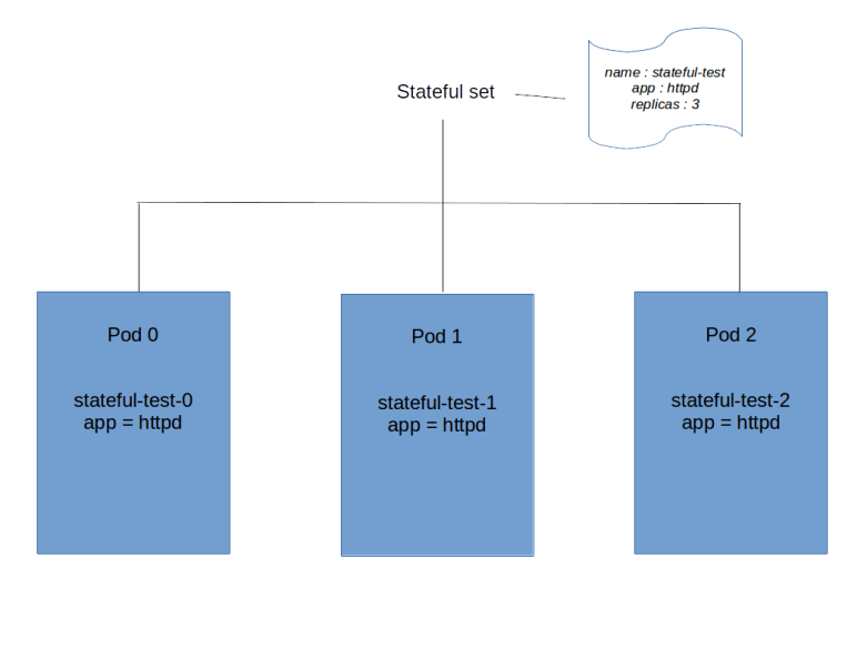
This is best explained using an example. So let us define a stateful set that contains three instances of a HTTPD (which, of course, is a toy example and not a typical application for which you would use stateful sets).

$ kubectl apply -f - << EOF
apiVersion: v1
kind: Service
metadata:
  name: httpd-svc
spec:
  clusterIP: None
  selector:
    app: httpd
---
apiVersion: apps/v1
kind: StatefulSet
metadata:
  name: stateful-test
spec:
  selector:
    matchLabels:
      app: httpd
  replicas: 3 
  serviceName: httpd-svc
  template:
    metadata:
      labels:
        app: httpd
    spec:
      containers:
      - name: httpd-ctr
        image: httpd:alpine
EOF
service/httpd-svc created
statefulset.apps/stateful-test created

That is a long manifest file, so let us go through it one by one. The first part of the file is simply a service called httpd-svc. The only thing that might seem strange is that this service has no cluster IP. This type of service is called a headless service. Its primary purpose is not to serve as a load balancer for pods (which would not make sense anyway in a typical stateful scenario, as the pods are not interchangeable), but to provide a domain in the cluster internal DNS system. We will get back to this point in a few seconds.

The second part of the manifest file is the specification of the actual stateful set. The overall structure is very similar to a deployment – there is the usual metadata section, a selector that selects the pods belonging to the set, a replica count and a pod template. However, there is also a reference serviceName to the headless service that we have just created.

Let us now inspect our cluster to see that this manifest file has created. First, of course, there is the service that the first part of our manifest file describes.

$ kubectl get svc httpd-svc
NAME        TYPE        CLUSTER-IP   EXTERNAL-IP   PORT(S)   AGE
httpd-svc   ClusterIP   None                     13s

As expected, there is no cluster IP address for this service and no port. In addition, we have created a stateful set that we can inspect using kubectl.

$ $ kubectl get statefulset stateful-test
NAME            READY   AGE
stateful-test   3/3     88s

The output looks similar to a deployment – we see that our stateful set has three replicas out of three in total in status READY. Let us inspect those pods. We know that, by definition, our stateful set consists of all pods that have an app label with value equal to httpd, so we can use a label selector to list all these pods.

$ kubectl get pods -l app=httpd 
NAME              READY   STATUS    RESTARTS   AGE
stateful-test-0   1/1     Running   0          4m28s
stateful-test-1   1/1     Running   0          4m13s
stateful-test-2   1/1     Running   0          4m11s

So there are three pods that belong to our set, all in status running. However, note that the names of the pods follow a different pattern than for a deployment. The name is composed of the name of the stateful set plus an ordinal, starting at zero. Thus the names are predictable. In addition, the AGE field tells you that Kubernetes will also bring up the pods in this order, i.e. it will start pod stateful-test-0, wait until this pod is ready, then bring up the second pod and so on. If you delete the set again, it will bring them down in the reverse order.

Let us check whether the pod names are not only predictable, but also stable. To do this, let us bring down one pod.

$ kubectl delete pod stateful-test-1
pod "stateful-test-1" deleted
$ kubectl get pods -l app=httpd 
NAME              READY   STATUS              RESTARTS   AGE
stateful-test-0   1/1     Running             0          8m41s
stateful-test-1   0/1     ContainerCreating   0          2s
stateful-test-2   1/1     Running             0          8m24s

So Kubernetes will bring up a new pod with the same name again – our names are stable. The IP addresses, however, are not guaranteed to remain stable and typically change if a pod dies and a substitute is created. So how would the pods in the set communicate with each other, and how would another pod communicate with one of them?

To solve this, Kubernetes will add DNS records for each pod. Recall that as part of a Kubernetes cluster, a DNS server is running (with recent versions of Kubernetes, this is typically CoreDNS). Kubernetes will mount the DNS configuration file /etc/resolv.conf into each of the pods so that the pods use this DNS server. For each pod in a stateful set, Kubernetes will add a DNS record. Let us use the busybox image to show this record.

$ kubectl run -i --tty --image busybox:1.28 busybox --restart=Never --rm
If you don't see a command prompt, try pressing enter.
/ # cat /etc/resolv.conf
nameserver 10.245.0.10
search default.svc.cluster.local svc.cluster.local cluster.local
options ndots:5
/ # nslookup stateful-test-0.httpd-svc
Server:    10.245.0.10
Address 1: 10.245.0.10 kube-dns.kube-system.svc.cluster.local

Name:      stateful-test-0.httpd-svc
Address 1: 10.244.0.108 stateful-test-0.httpd-svc.default.svc.cluster.local

What happens? Apparently Kubernetes creates one DNS record for each pod in the stateful set. The name of that record is composed of the pod name, the service name, the namespace in which the service is defined (the default namespace in our case), the subdomain svc in which all entries for services are stored and the cluster domain. Kubernetes will also add a record for the service itself.

/ # nslookup httpd-svc
Server:    10.245.0.10
Address 1: 10.245.0.10 kube-dns.kube-system.svc.cluster.local

Name:      httpd-svc
Address 1: 10.244.0.108 stateful-test-0.httpd-svc.default.svc.cluster.local
Address 2: 10.244.0.17 stateful-test-1.httpd-svc.default.svc.cluster.local
Address 3: 10.244.1.49 stateful-test-2.httpd-svc.default.svc.cluster.local

So we find that Kubernetes has added additional A records for the service, corresponding to the three pods that are part of the stateful set. Thus an application could either look up one of the services directly, or use round-robin and a lookup of the service name to talk to the pods.

As a sidenote, you have really have to use version 1.28 of the busybox image to make this work – later versions seem to have a broken nslookup implementation, see this issue for details.

Stateful sets and storage

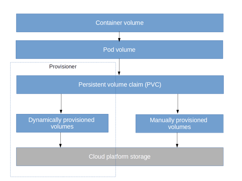
Stateful sets are meant to be used for applications that store a state, and of course they typically do this using persistent storage. When you create a stateful set with three replicas, you would of course want to attach storage to each of them, but of course you want to use different volumes. In case a pod is lost and restarted, you would also want to automatically attach the pod to the same volume to which the pod it replaces was attached. All this is done using PVC templates.

Essentially, a PVC template has the same role for storage that a pod specification template has for pods. When Kubernetes creates a stateful set, it will use this template to create a set of persistent volume claims, one for each member of the set. These persistent volume claims are then bound to volumes, either manually created volumes or dynamically provisioned volumes. Here is an extension of our previously used example that includes PVC templates.

apiVersion: v1
kind: Service
metadata:
  name: httpd-svc
spec:
  clusterIP: None
  selector:
    app: httpd
---
apiVersion: apps/v1
kind: StatefulSet
metadata:
  name: stateful-test
spec:
  selector:
    matchLabels:
      app: httpd
  replicas: 3 
  serviceName: httpd-svc
  template:
    metadata:
      labels:
        app: httpd
    spec:
      containers:
      - name: httpd-ctr
        image: httpd:alpine
        volumeMounts:
        - name: my-pvc
          mountPath: /test
  volumeClaimTemplates:
  - metadata:
      name: my-pvc
    spec:
      accessModes:
      - ReadWriteOnce
      resources:
        requests:
          storage: 1Gi

The code is the same as above, with two differences. First, we have an additional array called volumeClaimTemplates. If you consult the API reference, you will find that the elements of this array are of type PersistentVolumeClaim and therefore follow the same syntax rules as the PVCs discussed in my previous posts.

The second change is that in the container specification, there is a mount point. This mount point refers directly to the PVC name, not using a volume on Pod level as a level of indirection as for ordinary deployments.

When we apply this manifest file and display the existing PVCs, we will find that for each instance of the stateful set, Kubernetes has created a PVC.

$ kubectl get pvc
NAME                     STATUS   VOLUME                                     CAPACITY   ACCESS MODES   STORAGECLASS   AGE
my-pvc-stateful-test-0   Bound    pvc-78bde820-53e0-11e9-b859-0afa21a383ce   1Gi        RWO            gp2            1m
my-pvc-stateful-test-1   Bound    pvc-8790edc9-53e0-11e9-b859-0afa21a383ce   1Gi        RWO            gp2            38s
my-pvc-stateful-test-2   Bound    pvc-974cc9fa-53e0-11e9-b859-0afa21a383ce   1Gi        RWO            gp2            12s

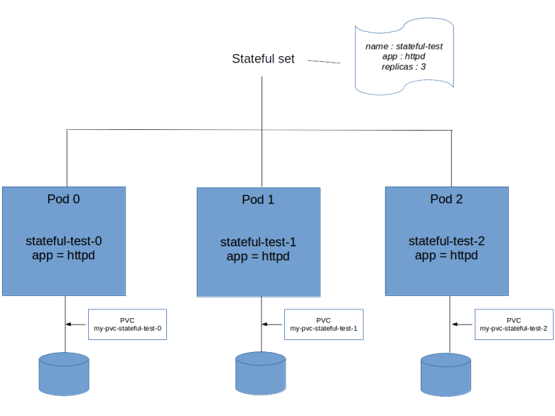
We see that again, the naming of the PVCs follows a predictable patterns and is composed of the PVC template name and the name of the corresponding pod in the stateful set. Let us now look at one of the pods in greater detail.

$ kubectl describe pod stateful-test-0
Name:               stateful-test-0
Namespace:          default
Priority:           0
[ --- SOME LINES REMOVED --- ]
Containers:
  httpd-ctr:
[ --- SOME LINES REMOVED --- ]
    Mounts:
      /test from my-pvc (rw)
      /var/run/secrets/kubernetes.io/serviceaccount from default-token-kfwxf (ro)
[ --- SOME LINES REMOVED --- ]
Volumes:
  my-pvc:
    Type:       PersistentVolumeClaim (a reference to a PersistentVolumeClaim in the same namespace)
    ClaimName:  my-pvc-stateful-test-0
    ReadOnly:   false
  default-token-kfwxf:
    Type:        Secret (a volume populated by a Secret)
    SecretName:  default-token-kfwxf
    Optional:    false
[ --- SOME LINES REMOVED --- ]

Thus we find that Kubernetes has automatically created a volume called my-pvc (the name of the PVC template) in each pod. This pod volume then refers to the instance-specific PVC which again refers to the volume, and this pod volume is in turn referenced by the Docker mount point.

What happens if a pod goes down and is recreated? Let us test this by writing an instance specific file onto the volume mounted by pod #0, deleting the pod, waiting for a few seconds to give Kubernetes enough time to recreate the pod and checking the content of the volume.

$ kubectl exec -it stateful-test-0 touch /test/I_am_number_0
$ kubectl exec -it stateful-test-0 ls /test
I_am_number_0  lost+found
$ kubectl delete pod stateful-test-0 && sleep 30
pod "stateful-test-0" deleted
$ kubectl exec -it stateful-test-0 ls /test
I_am_number_0  lost+found

So we see that in fact, Kubernetes has bound the same volume to the replacement for pod #0 so that the application can access the same data again. The same happens if we forcefully remove the node – the volume is then automatically attached to the node on which the replacement pod will be scheduled. Note, however, that this only works if the new node is in the same availability zone as the previous node as on most cloud platforms, cross-AZ attachment of volumes to nodes is not possible, in this case, the scheduler will have to wait until a new node in that zone has been brought up (see e.g. this link for more information on running Kubernetes in multiple zones).

Let us continue to investigate the life cycle of our volumes. We have seen that the volumes have been created automatically when the stateful set was created. The converse, however, is not true.

$ kubectl delete statefulset stateful-test
statefulset.apps "stateful-test" deleted
$ kubectl delete svc httpd-svc
service "httpd-svc" deleted
$ kubectl get pvc
NAME                     STATUS   VOLUME                                     CAPACITY   ACCESS MODES   STORAGECLASS   AGE
my-pvc-stateful-test-0   Bound    pvc-78bde820-53e0-11e9-b859-0afa21a383ce   1Gi        RWO            gp2            14m
my-pvc-stateful-test-1   Bound    pvc-8790edc9-53e0-11e9-b859-0afa21a383ce   1Gi        RWO            gp2            13m
my-pvc-stateful-test-2   Bound    pvc-974cc9fa-53e0-11e9-b859-0afa21a383ce   1Gi        RWO            gp2            13m

So the persistent volume claims (and the volumes) remain existent if the delete the stateful set. This seems to be a deliberate design decision to give the administrator a chance to copy or backup the data on the volumes even after the set has been deleted. To fully clean up the volumes, we therefore need to delete the PVCs manually. Fortunately, this can again be done using a label selector, in our case

kubectl delete pvc -l app=httpd

will do the trick. Note that it is even possible to reuse the PVCs – in fact, if you recreate the stateful set and the PVCs still exists, they will be reused and attached to the new pods.

This completes our overview of stateful sets in Kubernetes. Running stateful applications in a distributed cloud environment is tricky, and there is much more that needs to be considered. To see a few examples, you might want to look at some of the examples which are part of the Kubernetes documentation, for instance the setup of a distributed key-value store like ZooKeeper. You might also want to learn about operators that provide application specific controller logic, for instance promoting a database replica to a master if the current master node goes down. For some additional considerations on running stateful applications on Kubernetes you might want to read this nice post that explains additional mechanisms like leader elections that are common ingredients for a stateful distributed application.

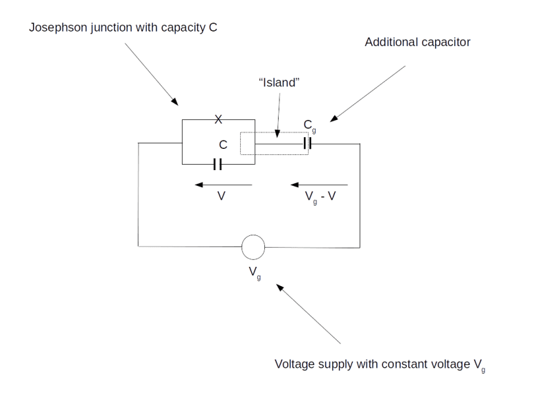
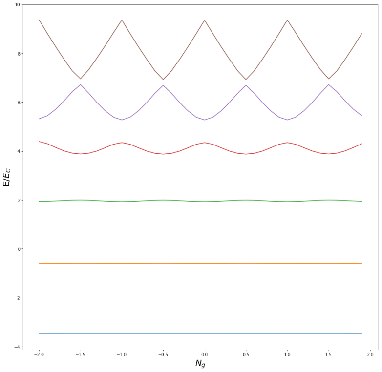
Superconducting qubits – on islands, charge qubits and the transmon

In my previous post on superconducting qubits, we have seen how a flux qubit represents a qubits state as a superposition of currents in a superconducting loop. Even though flux qubits have been implemented and used successfully, most research groups today focus on different types of qubits using a charge qubit as an archetype.

Charge qubits – the basics

The basic idea of a superconducting charge qubit is to create a small superconducting area called the island which is connected to a circuit in such a way that we can control the number of charge carries that are located on the island. A typical way to do this is shown in the diagram below.

In this diagram, we see, in the upper left, a Josephson junction, indicated by the small cross. Recall that a Josephson junction consists of two superconducting electrodes separated by a thin insulator. Thus a Josephson junction has a capacity, which is indicated by the capacitor C in the diagram.

On the right of the Josephson junction is a second capacitor. Now charge carriers, i.e. Cooper pairs, can tunnel through the Josephson junction and reach the area between the second capacitor and the junction – this is our island. Conversely, Cooper pairs can cross the junction to leave the island again. The flow of Cooper pairs into the island and away from the island can be controlled by applying an external voltage V_g. Effectively, a certain number of Cooper pairs will be trapped on the island – this is why this circuit is sometimes called a Cooper pair box – but this number will be subject to quantum fluctuations due to tunneling through the junction. Roughly speaking, these fluctuations cause an oscillation which will give us energy levels, and we can use two of these energy levels to represent our qubit.

Let us try to understand how these energy levels look like. Again, I will try to keep things short and refer to my more detailed notes on GitHub for more details. The Hamiltonian for our system looks as follows.

$H = E_C[N - N_g] - E_0 \cos \delta$

Here, E_g and E₀ are energies that are determined by the geometry of the junction and the value of the capacities in the circuit, N is the number of Cooper pairs on the island, N_g is a number depending on the external voltage and $\delta$ is (proportional to) the flux through the junction. Thus N and $\delta$ are our dynamic variables, representing the number of Cooper pairs on the island and its change over time, whereas the other quantities are parameters determined by the circuit and the external voltage. As N_g depends on the external voltage and can therefore be changed easily, this is the parameter we will be using to tweak our qubit.

Using a computer algebra program (or this Python notebook), it is not difficult to obtain a numerical approximation of the eigenvalues of this operator (we can, for instance, represent the Hamiltonian as a matrix subject to an eigenbasis for N and calculate its eigenvalues after cutting off at a finite dimension). The diagram below shows the results for E₀ = 0.1 E_c.

We see that if N_g is an integer, there is a degeneracy between the first and second excited state. If, however, N_g is a half-integer, then this degeneracy is removed, and the first two energy levels are fairly well separated from the rest of the spectrum.

With this relation of the two energies E_C and E₀, the probability for a Cooper pair to tunnel through the Josephson junction is comparatively small. Thus, the fluctuations in the quantum number N are small, and the eigenstates of N are almost stationary and therefore almost energy eigenstates. As the energy levels are well separated, we can use the first two energy levels as a qubit. As the eigenstates of the operator representing the charge on the island are almost stationary states, this regime is called the charge regime and the resulting qubit is called the charge qubit.

The transmon

This is all nice, but in practice, there is still a problem. To understand this, let us take a look at the energy level diagram above again. The energy levels are not flat, meaning that a change in the value of N_g is changing the energy levels and therefore the stationary states. Unfortunately, the value of N g does not only depend on the external voltage V_g (which we can control), but also on charge noise, i.e. unwanted charge fluctuations that are hard to suppress.

Therefore, the charge qubit is quite sensitive to charge noise. The point N_g = 0.5, called the sweet spot, is typically chosen because at this point, at least the first derivative of the energy as a function of the charge vanishes, so that the qubit is only affected by charge noise to the second order. However, this dependency remains and limits the coherence time of the charge qubit.

One way to reduce the sensitivity to charge noise is to increase the ratio between E₀ and E_C . To understand what happens if we do this, take a look at the following diagram which displays the first few energy levels when this ratio is 5.0

We see that, compared to our first energy level diagram, the sensitivity to charge noise is reduced, as the energy of the first two energy levels is almost flat, with a minimal dependency on N_g . However, this comes at the cost of a more equidistant spacing of the energy levels, making the isolation between the first two energy levels and the rest of the spectrum hard, and the question arises whether we gain an advantage at the cost of another one.

Fortunately, it turns out that the sensitivity to charge noise decreases exponentially fast, but the anharmonicity of the energy levels decreases much slower. Thus there is a region for the ratio E₀ / E_c in which this sensitivity is already comparatively low, but the energy levels are still sufficiently anharmonic to obtain a reasonable two-level system. A charge qubit operated in this regime is called a transmon qubit.

Technically, a larger value of E₀ compared to E_C is achieved by adding an additional capacitor parallel to the Josephson junction. If we use a high value for the additional capacity, we can make E_C arbitrarily small and can achieve an arbitrary high ratio of E₀ compared to E_C.

To develop a physical intuition of why this happens, recall that the energy E₀ of the Josephson junction measures the tunneling probability. If E₀ is large compared to E_C , it is comparatively easy for a Cooper pair to tunnel through the junction. Therefore the phase difference $\delta$ across the junction will only fluctuate slightly around a stationary value, i.e. the wave function will be localized sharply in the $\delta$ -space. Consequently, the charge N will no longer be a good quantum number and the charge eigenstates will no longer be approximate energy eigenstates. Instead, we will see significant quantum fluctuations in the charge, which makes the system more robust to external charge noise. In this configuration, you should therefore think of the qubit state not as a fixed number of Cooper pairs on the island, but more as a constant tunneling current flowing through the junction.

To control and read out a transmon qubit, it is common to use a parallel LC circuit which is coupled with the transmon via an additional capacitor. Using microwave pulses to create currents in that LC circuit, we can manipulate and measure the state of the qubit and couple different qubits. Physically, the LC circuit is realized as a transmission line resonator, in which – similar to an organ pipe – waves are reflected at both ends and create standing wave patterns (that transmission lines are used is the reason for the name transmon qubit).

At the time of writing, most major players (Google, IBM, Rigetti) are experimenting with transmon based qubit designs, as it appears that this type of qubit is most likely to be realizable at scale. In fact, Transmon qubits are the basic building blocks of Google’s Bristlecone architecture as well as for IBMs Q experience and Rigettis QPU.

To learn more, I recommend this and this review paper, both of which are freely available on the arXiv.

Kubernetes storage under the hood part III – storage classes and provisioning

In the last post, we have seen the magic of persistent volume claims in action. In this post, we will look in more details at how Kubernetes actually manages storage.

Storage classes and provisioners

First, we need to understand the concept of a storage class. In a typical environment, there are many different types of storage. There could be some block storage like EBS or a GCE persistent disk, or some local storage like an SSD or a HDD, NFS based storage or some distributed storage like Ceph or StorageOS. So far, we have kept our persistent volume claims platform agnostic, on the other hand, there might be a need to specify in more detail what type of storage we want. This is done using a storage class.

To start, let us use kubectl to list the available storage classes in our standard EKS cluster (you will get different results if you use a different provider).

$ kubectl get storageclass
NAME            PROVISIONER             AGE
gp2 (default)   kubernetes.io/aws-ebs   3h

In this case, there is only one storage class called gp2. This is marked as the default storage class, meaning that in case we define a PVC which does not explicitly refer to a storage class, this class is chosen. Using kubectl with one of the flags --output json or --output yaml, we can get more information on the gp2 storage class. We find that there is an annotation storageclass.kubernetes.io/is-default-class which defines whether this storage class is the default storage class. In addition, there is a field provisioner which in this case is kubernetes.io/aws-ebs.

This looks like a Kubernetes provided component, so let us try to locate its source code in the Kubernetes GitHub repository. A quick search in the source tree will show you that there is a fact a manifest file defining the storage class gp2. In addition, the source tree contains a plugin which will communicate with the AWS cloud provider to manage EBS block storage.

The inner workings of this are nicely explained here. Basically, the PVC controller will use the storage class in the PVC to find the provisioner that is supposed to be used for this storage class. If a provisioner is found, it is asked to create the requested storage dynamically. If no provisioner is found, the controller will just wait until storage becomes available. An external provisioner can periodically scan unmatched volume claims and provision storage for them. It then creates a corresponding persistent storage object using the Kubernetes API so that the PVC controller can detect this storage and bind it to the claim. If you are interested in the details, you might want to take a look at the source code of the external provisioner controller and the example of the Digital Ocean provisioner using it.

So at the end of the day, the workflow is as follows.

A user creates a PVC
If no storage class is provided in the PVC, the default storage class is merged into the PVC
Based on the storage class, the provisioner responsible for creating the storage is identified
The provisioner creates the storage and a corresponding Kubernetes PV object
The PVC is bound to the PV and available for use in Pods

Let us see how we can create our own storage classes. We have used the AWS EBS provisioner to create GP2 storage, but it does in fact support all storage types (gp2, io1, st1, sc1) offered by Amazon. Let us create a storage class which we can use to dynamically provision HDD storage of type st1.

$ kubectl apply -f - << EOF
apiVersion: storage.k8s.io/v1
kind: StorageClass
metadata:
  name: st1
provisioner: kubernetes.io/aws-ebs
parameters:
  type: st1
EOF
storageclass.storage.k8s.io/st1 created
$ kubectl get storageclass
NAME            PROVISIONER             AGE
gp2 (default)   kubernetes.io/aws-ebs   17m
st1             kubernetes.io/aws-ebs   15s

When you compare this to the default class, you will find that we have dropped the annotation which designates this class as default – there can of course only be one default class per cluster. We have again used the aws-ebs provisioner, but changed the type field to st1. Let us now create a persistent storage claim using this class.

$ kubectl apply -f - << EOF
apiVersion: v1
kind: PersistentVolumeClaim
metadata:
  name: hdd-pvc
  namespace: default
spec:
  accessModes:
    - ReadWriteOnce
  storageClassName: st1
  resources:
    requests:
      storage: 500Gi
EOF

If you submit this, wait until the PV has been created and then use aws ec2 describe-volumes, you will find a new AWS EBS volume of type st1 with a capacity of 500 Gi. As always, make sure to delete the PVC again to avoid unnecessary charges for that volume.

Manually provisioning volumes

So far, we have used a provisioner to automatically provision storage based on storage claims. We can, however, also provision storage manually and bind claims to it. This is done as usual – using a manifest file which describes a resource of kind PersistentVolume. To be able to link this newly created volume to a PVC, we first need to define a new storage class.

$ kubectl apply -f - << EOF
apiVersion: storage.k8s.io/v1
kind: StorageClass
metadata:
  name: cold
provisioner: kubernetes.io/aws-ebs
parameters:
  type: sc1
EOF
storageclass.storage.k8s.io/cold created

Once we have this storage class, we can now manually create a persistent volume with this storage class. The following commands create a new volume with type sc1, retrieve its volume id and create a Kubernetes persistent volume linked to that EBS volume.

$ volumeId=$(aws ec2 create-volume --availability-zone=eu-central-1a --size=1024 --volume-type=sc1  --query 'VolumeId')
$ kubectl apply -f - << EOF
apiVersion: v1
kind: PersistentVolume
metadata:
  name: cold-pv
spec:
  capacity:
    storage: 1024Gi
  accessModes:
    - ReadWriteOnce
  storageClassName: cold
  awsElasticBlockStore:
    volumeID: $volumeId
EOF

Initially, this volume will be available, as there is no matching claim. Let us now create a PVC with a capacity of 512 Gi and a matching storage class.

$ kubectl apply -f - << EOF
apiVersion: v1
kind: PersistentVolumeClaim
metadata:
  name: cold-pvc
  namespace: default
spec:
  accessModes:
    - ReadWriteOnce
  storageClassName: cold
  resources:
    requests:
      storage: 512Gi
EOF

This will create a new PVC and bind it to the existing persistent volume. Note that the PVC will consume the entire 1 Ti volume, even though we have only requested half of that. Thus manually pre-provisioning volumes can be rather inefficient if the administrator and the teams do not agree on standard sizes for persistent volumes.

If we delete the PVC again, we see that persistent volume is not automatically deleted, as it was the case for dynamic provisioning, but survices and can be consumed again by a new matching claim. Similarly, deleting the PV will not automatically delete the underlying EBS volume, and we need to clean up manually.

Using Python to create volume claims

As usual, we close this post with some remarks on how to use Python to create and use persistent volume claims. Again, we omit the typical boilerplate code an refer to the full source code on GitHub for all the details.

First, let us look at how to create and populate a Python object that corresponds to a PVC. We need to instantiate an instance of V1PersistentVolumeClaim. This object again has the typical metadata, contains the access mode and a resource requirement.

pvc=client.V1PersistentVolumeClaim()
pvc.api_version="v1"
pvc.metadata=client.V1ObjectMeta(
                  name="my-pvc")
spec=client.V1PersistentVolumeClaimSpec()
spec.access_modes=["ReadWriteOnce"]
spec.resources=client.V1ResourceRequirements(
                  requests={"storage" : "32Gi"})
pvc.spec=spec

Once we have this, we can submit an API request to Kubernetes to actually create the PVC. This is done using the method create_namespaced_persistent_volume_claim of the API object. We can then create a pod specification that uses this PVC, for instance as part of a deployment. In this template, we first need a container specification that contains the mount point.

container = client.V1Container(
                name="alpine-ctr",
                image="httpd:alpine",
                volume_mounts=[client.V1VolumeMount(
                    mount_path="/test",
                    name="my-volume")])

In the actual Pod specification, we also need to populate the field volumes. This field contains a list of volumes, which again refer to a volume source. So we end up with the following code.

pvcSource=client.V1PersistentVolumeClaimVolumeSource(
              claim_name="my-pvc")
podVolume=client.V1Volume(
              name="my-volume",
              persistent_volume_claim=pvcSource)
podSpec=client.V1PodSpec(containers=[container], 
                         volumes=[podVolume])

Here the claim name links the volume to our previously defined PVC, and the volume name links the volume to the mount point within the container. Starting from here, the creation of a Pod using this specification is then straightforward.

This completes our short series on storage in Kubernetes. In the next post on Kubernetes, we will look at a typical application of persistent storage – stateful applications.

Kubernetes storage under the hood part II – persistent storage

The storage types that we have discussed so far realize ephemeral storage, i.e. storage tied to the lifecycle of the Pod on a specific node. Of course, there are many use cases like databases or other stateful applications that require storage that is persistent and has a lifecycle independent of the Pod. In this post, we look at different ways to realize this in Kubernetes.

Using cloud provider specific storage directly

The easiest – and historically first – way to do this is to directly refer to an existing piece of persistent storage provided by the underlying cloud platform. Recall that when you define and use volumes, you define the volume as part of Pod specification, assign a name and tell Kubernetes which type of volume it should allocate – like emptyDir or hostPath. If you check the list of supported volumes, you will find some volumes that are specific to a cloud provider, for instance awsElasticBlockStore. This allows you to mount a pre-existing AWS Elastic Block Store volume into your Pod. As EBS volumes can only be attached to one instance at a time, you can only connect to this volume from one Pod.

To try this out, we of course have to generate an EBS volume first (as always, be aware of the charges and make sure to delete the volume if it is no longer needed). EBS volumes need to be created within an availability zone (which you can figure out using aws ec2 describe-availability-zones). In my example, I will use the availability zone eu-central-1a. The following command creates a 16 GiB GP2 (SSD) drive in this availability zone.

$ aws ec2 create-volume --availability-zone=eu-central-1a\
           --size=16 --volume-type=gp2

If you now run aws ec2 describe-volumes --output json to list all volumes, you will see several volumes that have the status “in-use” (these are the root volumes of your nodes) and one new volume that has the status “available”. We will need the volume ID of this volume, in my case this is vol-0eb2505d4b7d035cb. Let us try to attach this to a Pod using the following manifest file.

apiVersion: v1
kind: Pod
metadata:
  name: ebs-demo
  namespace: default
spec:
  containers:
  - name: ebs-demo-ctr
    image: httpd:alpine
    volumeMounts:
      - mountPath: /test
        name: test-volume
  volumes:
  - name: test-volume
    awsElasticBlockStore: 
      volumeID: vol-0eb2505d4b7d035cb

Sometimes you learn most from your mistakes. If you apply this manifest file chances are that your Pod will never be fully established, but will remain in the state “ContainerCreating” forever. What is going wrong?

To find the answer, use the AWS CLI or the AWS Web console to look at the availability zones of the instance on which the Pod is scheduled and the volume. In my example, Kubernetes did schedule the Pod on a node running in eu-central-1c, whereas the volume was created in eu-central-1a. Unfortunately, EBS volumes cannot be attached across availability zones, and the creation of the Pod fails.

Fortunately, there is a way out. Note that EKS will attach a label to the nodes which capture there availability zone. This label is called failure-domain.beta.kubernetes.io/zone. Now, Kubernetes has a general mechanism called node selector. This allows you to instruct the Kubernetes scheduler to move Pods only on specific nodes, matching certain selection criteria. These criteria are provided in the section nodeSelector of the Pod specification. So the following updated manifest file makes sure that the node will be scheduled in the availability zone in which we did create the volume.

apiVersion: v1
kind: Pod
metadata:
  name: ebs-demo
  namespace: default
spec:
  containers:
  - name: ebs-demo-ctr
    image: httpd:alpine
    volumeMounts:
      - mountPath: /test
        name: test-volume
  volumes:
  - name: test-volume
    awsElasticBlockStore: 
      volumeID: vol-0eb2505d4b7d035cb
  nodeSelector:
    failure-domain.beta.kubernetes.io/zone: eu-central-1a

If you apply this manifest file and wait for some time, you will see that the Pod comes up. If you again run aws ec2 describe-volumes, you will find that the volumes status has changed to “in-use” and that EKS has automatically attached it to the node on which the Pod is scheduled (provided, of course, that you have a node running in eu-central-1a, which is not a given if you only use two nodes as we do it – in this case you will have to create the volume in one of the availability zones in which you have a node). You can also attach to the Pod and run mount to verify that a device has been mounted on /test. Combining the output of docker inspect and mount on the node will tell you that the following has happened.

Kubernetes has asked AWS to attach our volume as /dev/xvdba to the node
Then Kubernetes did create a directory specific to the Pod
The volume was mounted into this directory
Finally, Kubernetes did create a Docker bind mount to hook up this directory on the node with the directory /test in the container file system

This example nicely demonstrates that using existing persistent storage in the underlying cloud platform is possible, but comes with some drawbacks. An administrator will have to manage these volumes manually, using whatever tools your cloud provider makes available. There are limitations if your cluster is spanning multiple availability zones, and of course you tie all your manifest files directly to a specific cloud provider. In addition, Kubernetes tries to follow the idea of “run everywhere”, which does not combine well with an approach where each individual cloud provider needs to be hardcoded into the core Kubernetes code base. As so often in computer science, this situation almost cries for an additional abstraction layer between Pod volumes and the underlying storage. This abstraction layer exists and is the topic of the next section.

Persistent volume claims

In the previous section, we have defined volumes as part of a Pod specification. These volumes – which we should actually call Pod volumes – are linked to the lifecycle of an individual Pod. We have seen that these volumes can refer to existing storage within your cloud layer, but that this comes with some drawbacks and requires manual provisioning outside of the Kubernetes world.

To change this, Kubernetes defines an additional abstraction layer between the storage as provided by the cloud platform and the Pod volumes. The most important objects we need to discuss in order to understand this are persistent volumes (PV) and persistent volume claims (PVC).

Let us start with persistent volumes. Essentially, a persistent volume is a Kubernetes object that represents a piece of storage in the underlying cloud platform. Typically, volumes are created dynamically, but we will see in the next post in this series that they can also be managed manually. The important thing is that volumes are first-class Kubernetes citizens and have a lifecycle independent of that of Pods.

Volumes represent the supply side of storage on your cluster. The demand side is represented by volume claims. A persistent volume claim is an object that a user creates to let Kubernetes know that a certain amount of storage is required. If the cluster is set up for it, Kubernetes will then automatically try to fulfill the claim, i.e. to either find an existing, unused volume that matches the claim or to provision a volume dynamically, using a so-called provisioner. A persistent volume claim can then be referenced in a Pod volume which in turn can be mounted into a container.

To get an idea what this means, let us again consider an example. The following manifest file describes a persistent volume claim.

apiVersion: v1
kind: PersistentVolumeClaim
metadata:
  name: ebs-pvc
  namespace: default
spec:
  accessModes:
    - ReadWriteOnce
  resources:
    requests:
      storage: 4Gi

In addition to the standard fields, we have a specification that consists of two sections. The first section specifies the access mode. Here we use ReadWriteOnce, which states that we want a volume which can be accessed by one Pod at a time, reading and writing. In the second section, we specify the resources, i.e. the amount of storage that we need, in our case 4 Gigabytes of storage. This example already demonstrates one nice feature of a PVC – it does not refer at all to a specific type of volume or a specific cloud platform (it does so indirectly, via the mechanism of storage classes, which we will investigate in the next post).

When we apply this manifest file and wait for a few seconds, we can look at the objects that have been created. First, run kubectl get pvc to get a list of all persistent volume claims.

$ kubectl get pvc
NAME      STATUS   VOLUME                                     CAPACITY   ACCESS MODES   STORAGECLASS   AGE
ebs-pvc   Bound    pvc-63521bd7-4e51-11e9-8e51-0af6f9d0ca50   4Gi        RWO            gp2            7m

So as expected, we have a new persistent volume claim that has been generated. The status of this PVC is “bound”, telling us that the provisioner working behind the scenes was able to find a matching volume. We also find a reference to the volume in the output. So let us list this volume.

$ kubectl get pv
NAME                                       CAPACITY   ACCESS MODES   RECLAIM POLICY   STATUS   CLAIM             STORAGECLASS   REASON   AGE
pvc-63521bd7-4e51-11e9-8e51-0af6f9d0ca50   4Gi        RWO            Delete           Bound    default/ebs-pvc   gp2

As stated above, this volume exists as an independent entity that we can refer to by its name and that has some properties. When we append --output json to get all the details, we see a few interesting things.

First, the volume has a field claimRef which tells us to which claim this volume is bound. This is only one field, not an array. Similarly, the PVC has a field volumeName referring to the underlying volume, which is again not an array. So the relation between a PV and a PVC is one-to-one. As mentioned in the documentation, this can lead to overprovisioning. If, for instance, you request 4 Gi, and there is a free volume with 8 Gi, the provisioner might decide to bind the PVC to this volume, even though only 4 Gi were requested.

Another interesting information that we get from the JSON output is that a volume has a label that tells us in which availability zone the volume (or, more precisely, the underlying EBS volume) is located. And, finally, the spec section contains a field that lets us locate the underlying EBS storage. You can use the following statements to extract this information and use the AWS CLI to print out some details of this volume.

$ fullVolumeID=$(kubectl get pv\
            --output=jsonpath='{.items[0].spec.awsElasticBlockStore.volumeID}')
$ volumeID=$(echo $fullVolumeID | sed 's/aws:\/\/.*\///')
$ aws ec2 describe-volumes --volume-id=$volumeID --output json

Let us now actually use this volume, i.e. attach it to a Pod. Here is a manifest file which will bring up a Pod mounting this volume.

apiVersion: v1
kind: Pod
metadata:
  name: pv-demo
  namespace: default
spec:
  containers:
  - name: pv-demo-ctr
    image: httpd:alpine
    volumeMounts:
      - mountPath: /test
        name: test-volume
  volumes:
  - name: test-volume
    persistentVolumeClaim:
      claimName: ebs-pvc

We see that at the point in the file were we did previously refer directly to an EBS volume, we now refer to the PVC. So again, there is no EBS or EKS specific data in this manifest file, and we can theoretically use the same manifest file on any cloud platform.

When you apply this manifest file, you will notice that it takes significantly longer for the containers to come up, this is because behind the scenes, Kubernetes needs to attach the EBS volume to the node on which the Pod is scheduled, which takes some time.

We can now again analyze the structure of the file systems in the container and on the node. If we do this, we will find a very similar picture as above. The container has a bind mount into a directory managed by Kubernetes. This directory in turn is a mount point for the device /dev/xvdbu. If we look at the output of aws ec2 describe-volumes, we find that this is the device to which AWS has attached the EBS volume behind the PVC. So the outcome of the entire exercise is the same as before, with the difference that no manual provisioning of the volume as necessary.

In addition, Kubernetes is smart enough to place our Pod in a the same availability zone in which the volume is located. In fact, as explained in the documentation on multi-zone capabilities, the Kubernetes scheduler will make sure that a Pod that requires a PV located in a given availability zone will only be placed on a node running in that zone. It can, however, happen that a volume is created in an availability zone where there is no node at all, rendering it unusable (see this GitHub issue for a discussion).

Let us now investigat the lifecycle of this storage. To do this, let us create a file in our newly mounted directory, kill the pod, bring it up again and list the contents of the volume (this assumes that you have saved the manifest file for the Pod in a file called pvUsage.yaml).

$ kubectl exec -it pv-demo touch /test/hello
$ kubectl delete pod pv-demo
pod "pv-demo" deleted
$ kubectl apply -f pvUsage.yaml
pod/pv-demo created
$ # Wait for container to be ready
$ kubectl exec -it pv-demo ls /test
hello       lost+found

So, as expected, the volume and its content have survived the restart of the Pod. If a persistent volume claim is deleted, however, Kubernetes will automatically delete the underlying volume and delete the corresponding storage in the cloud platform layer. When you shutdown a cluster, make sure to delete all PVCs first, otherwise orphaned block storage volumes not controlled by Kubernetes any more could result.

We have now covered the basics of persistent storage in Kubernetes – but of course there is much more that we have still left open. How is storage actually provisioned? How does the platform know which type of storage we need when we issue a PVC? And how can we manually create storage? These are the topics that we will discuss in the next post in this series.

Superconducting qubits – the flux qubit

In the last post, we have discussed the basic idea of superconducting qubits – implement circuits in which a supercurrent flows that can be described by a quantum mechanical wave function, and use two energy levels of the resulting quantum system as a qubit. Today, we will look in some more detail into one possible realization of this idea – flux qubits.

In its simplest form, a flux qubit is a superconducting loop threaded by an external magnetic field and interrupted by a Josephson junction. This is visualized on the left hand side of the diagram below, while the right hand side shows an equivalent circuit, formed by an inductance L, the capacity C_J of the junction and the pure junction.

It is not too difficult to describe this system in the language of quantum mechanics. Essentially, its state at a given point in time can be described by two quantities – the charge stored in the capacitor formed by the two leads of the Josephson junction, and the magnetic flow (or flux) through the loop. If you carefully go through all the details and write down the resulting equation for the Hamiltonian, you will find that the classical equivalent of this system is a particle moving in a potential which, for an appropriate choice of the parameters of the circuit, looks like the one displayed below.

This potential has a form which physicists call a double-well potential. Let us discuss the behavior of a particle moving in such a potential qualitatively. Classically, the particle would eventually settle down at one the minima. As long as its energy is below the height of the potential separating these two minima, it would remain in that state. In the quantum world, however, we would expect tunneling to occur, i.e. we would expect that our system has two basic states, one corresponding to the particle being close the left minimum and one corresponding to the particle being right to the minimum, and that we see a certain non-zero probability for the particle to cross the potential wall and to flip from one state into the other state. This two-state system already looks like a good candidate for a qubit.

Being a one-dimensional system, the eigenstate wave functions can be approximated numerically using standard methods, for example the “particle-in-a-box” approach. Again, I refer to my detailed notes for the actual calculation. The result is displayed below.

The diagram shows the ground state (blue curve on the left hand side) and the first excited state (blue curve on the right hand side). In both diagrams, I have added the classical potential (orange line) for the purpose of comparison. So we actually obtain the picture that we expect. Up to normalization, the ground state – the eigenstate on the left – is a superposition of two states

$|l \rangle - | r \rangle$

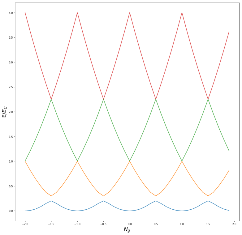
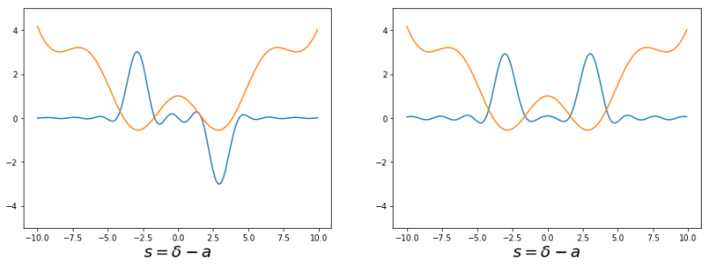
where $|l \rangle$ is a state localized around the left minimum of the potential and $|r \rangle$ is a state centered around the right minimum, whereas the first excited state is a linear combination proportional to

$|l \rangle + | r \rangle$

In general, there will be a small energy difference between these two states, which leads to a non-zero probability for tunneling between them. Intuitively, the state $|l \rangle$ corresponds to a supercurrent that flows through the loop in one direction and the state $|r \rangle$ is a state in which the supercurrent flows in the opposite direction. Our ground state – which would be the state $|0 \rangle$ in an interpretation as a qubit – and our first excited state $|1 \rangle$ are superpositions of these two states.

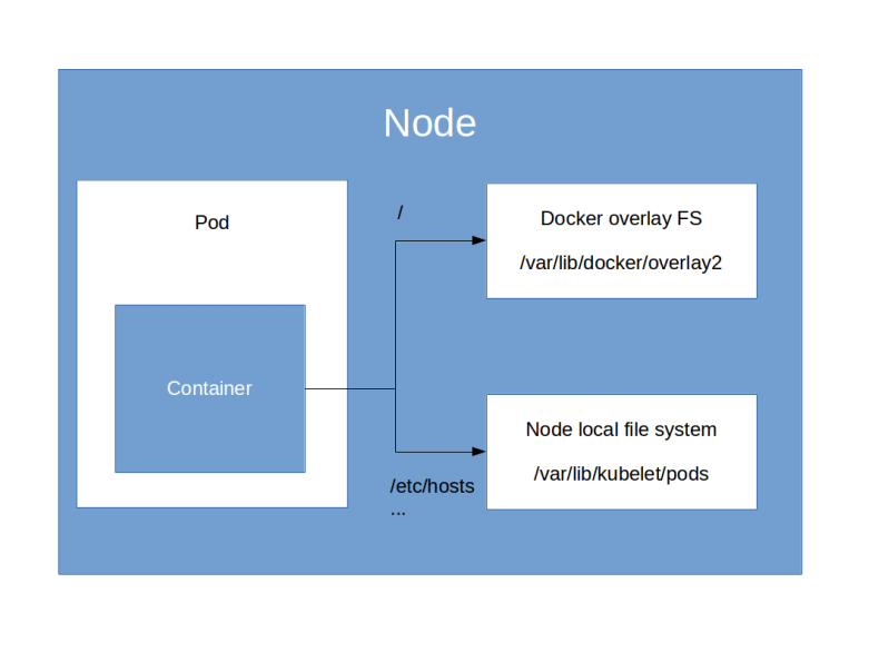
A nice property of the flux qubit is that the energy gap between the first excited state and the second excited state is much higher than the energy gap between the ground state and the first excited state. In the example used as basis for the numerical simulations described here, the second gap is more than one order of magnitude higher than the first gap. This implies that the two level system spanned by $|0 \rangle$ and $|1 \rangle$ is a fairly well isolated system and thus serves as a very good approximation to a qubit. The Hamiltonian can be manipulated by changing the flux through the loop by applying an external magnetic field or an external microwave pulse can be used to stimulate a transition from the ground state to the first excited state. In this way, the qubit can be read-out and controlled.

So theoretically, this system is a good candidate for the implementation of a qubit. In fact, this has been used in practice – the D-Wave quantum annealer is based on interconnected flux qubits. However, it seems that the flux qubit has come a bit out of fashion, and research has focussed on a new generation of superconducting qubits like the transmon qubit that work slightly differently. We will study this type of qubit in the next post in this series.

Kubernetes storage under the hood part I – ephemeral storage

So far, we have mainly discussed how compute and network resources are used and managed with Kubernetes. We will now turn to the third fundamental element of a container platform – storage.

Docker storage concepts

Before we talk about Kubernetes storage concepts, let us first recall how storage is managed in Docker. The following tests assume that you have a local installation of Docker on a Linux workstation (or virtual machine, of course). As a refresher, you might want to take a look at my introduction into Docker internals before reading on.

First, let us start a Docker container and spawn a shell. The easiest way to do this is the busybox image. So let us spin up a busybox container, attached to the terminal, and run mount to inspect its file system.

$ docker run -it busybox
/ # mount
overlay on / type overlay (rw,relatime,lowerdir=/var/lib/docker/overlay2/l/BNUAN2FS4K75ZLQFSZVQWXRLUU:/var/lib/docker/overlay2/l/UKEGOK4TLTD2T4XN5KIEPN7JXF,upperdir=/var/lib/docker/overlay2/e8f16f0d705fb8e4677b605796b7319ef3f0226e2ad173b506e13b479afa515f/diff,workdir=/var/lib/docker/overlay2/e8f16f0d705fb8e4677b605796b7319ef3f0226e2ad173b506e13b479afa515f/work)
proc on /proc type proc (rw,nosuid,nodev,noexec,relatime)
tmpfs on /dev type tmpfs (rw,nosuid,size=65536k,mode=755)
[REDACTED - SOME LINES REMOVED]

Your output will most likely look differently, but the general pattern will be the same. The first mount point that we see is the mount for the root directory. On newer Docker versions, this will be an overlay2 file system, on older Docker versions, it will be of type aufs. This entry points to one or more actual files on the host system that are located in the directory /var/lib/docker/ which is managed by Docker. These are the files in which the actual content of the root filesystem is stored.

The data on that file system is volatile and linked to the lifecycle of the container. To see this, let us create a file in the containers root file system and exit the container.

/ # echo "dancing in the rain" > /franky
/ # exit

This will stop the container, but not remove it – it will still exist and be visible in the output of docker ps -a. If you restart the container and attach to the running container, you will find that the file is still there and its content has been preserved. If, however, you remove the container using docker rm, the corresponding files on the host file system will be removed and the content of the file system of our container is lost. In that sense, these volumes are ephemeral – they survive across restarts, but die if the container is removed.

But Docker can do more – we can also use persistent storage. One option to do this are bind mounts. A bind mount maps a directory or a file from the host file system into the namespace of the container and attaches it to a mount point. To see an example, create a temporary directory on your host system and put some data into it. We can then mount this directory into a new Docker container using the -v option.

$ mkdir /tmp/ctr-test/
$ echo "Hello World" > /tmp/ctr-test/hello
$ docker run -v /tmp/ctr-test:/ctr-test/ -it busybox 
/ # cat /ctr-test/hello
Hello World
/# exit

So the content of the directory /tmp/ctr-test on the host becomes accessible within the container as /ctr-test (of course I could have chosen any other name as well). We can also see this mount point in the output of docker inspect. Use docker ps -a to find out the ID of the busybox container, in my case fd8ef21ba685, and then run

$ docker inspect fd8ef21ba685 --format="{{json .Mounts}}"
[{"Type":"bind","Source":"/tmp/ctr-test","Destination":"/ctr-test","Mode":"","RW":true,"Propagation":"rprivate"}]

So the mount point shows up as a mount point of type bind in the list of mounts of our container.

We remark that Docker also has a more advanced way to mount storage referred to as volumes. In contrast to a bind mount, a volume is an object managed by Docker, backed by files in the Docker controlled directories. Volumes can be created manually or dynamically, can be given a name and can be mounted into a container. As they are objects with an independent lifecycle, they survive container eviction and can be mounted to more than one container. However, we will not look deeper into this as (at least to my knowledge) this feature is not used by Kubernetes.

Ephemeral storage in Kubernetes

Now let us try out how things change if we use Kubernetes to spin up our containers.

$ kubectl run -i --tty busybox --image=busybox --restart=Never
/ # / # mount
overlay on / type overlay (rw,relatime,lowerdir=/var/lib/docker/overlay2/l/57X3FQLOLATAMPLAASUMBKHD5W:/var/lib/docker/overlay2/l/Q6HSQOG4NX7UHGVZEPQIZI43KQ,upperdir=/var/lib/docker/overlay2/f183dfd193c86bf43ebca4ae7d08cbfd6e268229f3bd59c70be2f48d9dc0937f/diff,workdir=/var/lib/docker/overlay2/f183dfd193c86bf43ebca4ae7d08cbfd6e268229f3bd59c70be2f48d9dc0937f/work)
[REDACTED]

So we see pretty much the same picture. The root volume of the container is again an overlay file system that is backed by directories managed by Docker on the host on which the pod is running.

If, however, you ssh into the node on which the container is running and do a docker inspect as before, you will find that there are actually a couple of bind mounts that we have not explicitly specified. These bind mounts are added by Kubernetes to give the container access to some configuration data like the token that can be used to connect to a Kubernetes service account, or host name resolutions (the own IP address of the container, for instance). Up to this point, our picture is actually quite simple.

Now things get a bit more complicated if you want to mount additional volumes. Kubernetes does in fact offer a large number of different volume types. Some of these volume types are ephemeral, i.e. the data is potentially lost if the pod dies or is rescheduled to a different node, other types of volumes are persistent. In this post, we focus on ephemeral storage and discuss different strategies to attach persistent storage in a later post.

Mount ephemeral storage of type emptyDir

In Kubernetes, we can define volumes on the level of an individual pod and attach these volumes to one or more containers that are running in this pod. Kubernetes offers several types of volumes. The type we are going to look at first is called an emptyDir because, from the point of view of a container, it is exactly that – a directory which is initially empty.

To see this in action, let us look at the following manifest file.

apiVersion: v1
kind: Pod
metadata:
  name: empty-dir-demo
  namespace: default
spec:
  containers:
  - name: empty-dir-demo-ctr
    image: httpd:alpine
    volumeMounts:
      - mountPath: /test
        name: test-volume
  volumes:
  - name: test-volume
    emptyDir: {}

This manifest file defines an individual Pod, as we have seen it before. However, there are a few new elements which are populated in this manifest. The Pod specification contains a new field volumes, which is an array of volume objects. This volume has a name and an additional field which indicates the type of the volume. The documentation lists many of them, here we are working with a volume of type emptyDir.

In the container specification, we now refer to this volume. This instructs Kubernetes to create the volume and to mount it into this container at the defined mount point. To see this in action, let us apply this manifest file, spawn a shell in the pod that is created and inspect its file system.

$ kubectl apply -f https://raw.githubusercontent.com/christianb93/Kubernetes/master/emptyDir.yaml 
pod/empty-dir-demo created
$ kubectl exec -it empty-dir-demo "/bin/bash"
bash-4.4# mount | grep "test"
/dev/xvda1 on /test type xfs (rw,noatime,attr2,inode64,noquota)

So we see that Kubernetes has actually mounted a new file system onto the mount point /test. To figure out how this is realized, let us take a closer look at the Docker container that has been created. So ssh into the node on which the Pod is running and run the following commands (this assumes that jq is installed on the node, which is the default when using the standard AWS AMI).

$ containerId=$(docker ps | grep "httpd" | awk '{print $1}')
$ docker inspect $containerId | jq -r '.[0].Mounts[]'
{
  "Type": "bind",
  "Source": "/var/lib/kubelet/pods/0914a859-4da2-11e9-931c-06a2d10ef1fe/volumes/kubernetes.io~empty-dir/test-volume",
  "Destination": "/test",
  "Mode": "",
  "RW": true,
  "Propagation": "rprivate"
}
[ ... more output ... ]

So we find that Kubernetes realizes an emptyDir volume as a bind mount, i.e. Kubernetes will create a directory on the nodes local file system and use a Docker bind mount to mount this into the container. Of course, this directory will initially be empty (as the name strongly suggests). Let us see what happens if we actually write something onto this file system. The following commands (to be run again on the node on which the Pod is running) extract the directory which is used for the bind mount from the output of docker inspect and list the contents of this directory.

$ dir=$(docker inspect $containerId | jq -r '.[0].Mounts[] | select(.Destination=="/test") | .Source')
$ sudo ls $dir

If you run this now, you will find that the directory is empty. Now switch back to the terminal attached to the Pod and create a file in the /test directory.

bash-4.4# echo "hello" > /test/hello

If you now list the directories content again, you will find that a file hello has been created.

Knowing how an emptyDir is implemented now makes it easy to understand the statements on the lifecycle in the Kubernetes documentation. It is stored in a directory specific for the Pod, i.e. it is initially created when the Pod is created and removed when the Pod is removed. It survices container restarts, but when the Pod is migrated to a different node, the content will be lost. In that sense, it is ephemeral storage.

Accessing host-local file systems

We have found that a volume of type emptyDir is nothing but a Docker bind mount to a Pod specific directory managed by Kubernetes. Of course, Kubernetes also offers a way to set up bind mounts to existing directories in the host file system (needless to say that this might be a security risk). This done using a volume of type hostPath as in the example below.

apiVersion: v1
kind: Pod
metadata:
  name: host-path-demo
  namespace: default
spec:
  containers:
  - name: host-path-demo-ctr
    image: httpd:alpine
    volumeMounts:
      - mountPath: /test
        name: test-volume
  volumes:
  - name: test-volume
    hostPath: 
      path: /etc

When you run this and attach to the resulting Pod, you will find that the content of the directory /test now match the content of the directory /etc on the host. Using again docker inspect on the node on which the Pod is running, you will find that Kubernetes has created an additional bind mount for the container which links the containers /test directory to the directory /etc on the host. Consequently, the contents of a hostPath volume will survive container restarts but will not be accessible anymore once the Pod is migrated to a different host.

Superconducting qubits – an introduction

In some of the last posts in my series on quantum computing, we have discussed how NMR (nuclear magnetic resonance) technology can be used to implement quantum computers. Over the last couple of years, however, a different technology has attracted significantly more interest and invest – superconducting qubits.

What are superconducting qubits? To start with something a bit more familiar, let us look at an analogue in classical electronics – an LC circuit. If you have ever built a transistor-based radio, you will have seen this. An LC circuit consists of an inductor and a capacitor, connected together as follows.

To understand what this circuit is doing, let us assume that at some point in time, the capacitor is fully charged. Then current will start to flow through the inductor. This will create a magnetic field in the inductor, so the electric energy stored in the capacitor is transformed into magnetic energy stored in the magnetic field of the inductor. Once the capacitor is fully decharged, the magnetic field will start to break down, again inducing a current which will then recharge the capacitor and so forth. This follows a pattern that every physicist knows by the name harmonic oscillator.

Now, in quantum mechanics, a harmonic oscillator has an infinite number of energy levels at equally spaced values. Can we use two of them, say the ground state and the first excited state, to build a qubit? Unfortunately there are a few obstacles.

The first problems is that an ordinary current is the coordinated movement of many electrons that constantly interact with the environment (dissipating heat due to the non-zero resistance) and therefore do not make a good closed quantum system. Even though each individual electron is of course a quantum mechanical system, the overall system exhibits classical behavior.

This changes if we use a superconducting LC circuit. As soon as we enter the superconducting regime, the flow of charge is no longer given by individual moving electrons, but by Cooper pairs that flow through the conductor. It is well known that in this state, the system can be described by a macroscopic wave function and is therefore behaving according to the laws of quantum mechanics, leading to phenomena like the quantization of the magnetic flux in a superconducting loop.

Does this mean that we can use a superconducting LC circuit, which then should behave as a quantum mechanical harmonic oscillator, as a qubit? Well, we are not quite there yet – as the energy levels of a harmonic oscillator are equally spaced, the first two levels are not well isolated against the remaining levels which makes it very hard to confine the system to these two levels.

Enter Josephson junctions. A Josephson junction is a superconducting element which consists of two superconducting solids that are separated by a thin insulator, like displayed schematically below.

Due to tunneling, Cooper pairs can cross the junction and thus a superconducting current can flow through the element. It turns out that a Josephson junction behaves like an inductor whose inductance is not constant (as for an ordinary inductor), but depends on the current. This will change the Hamiltonian of the system to the effect that the energy levels become distorted. If we get the parameters right, we are able to obtain a situation where the two lowest energy levels are separated fairly well from the rest of the energy spectrum and therefore the corresponding subsystem can approximately be treated as a two-level system, i.e. a qubit.

Superconducting qubits have gained a lot of attention over the last two years. They can be produced with techniques known from the production of integrated circuit, and they can be controlled with classical electronics. Their dimensions are within the realm of traditional IC technology, being in the micrometer range. The picture below (credits A. ter Haar, PhD thesis) shows a superconducting qubit (a so-called flux qubit) made of an inner loop with three Josephson junctions and an outer loop for readout and control.

qubit1 — picture taken from the PhD thesis of A. ter Haar

In addition, superconducting qubits can easily be layed out on a chip, which makes them good candidates for small, highly integrated quantum computing devices. Of course they need cooling as the need to operate below the critical temperature of the employed superconducting material, but this is standard technology by now. Today, most of the big players in the quantum world like Google, IBM, Rigetti and D-Wave are focusing their efforts on superconducting qubits.

To interact with the qubit (and to make two qubits interact), there are several options. We can apply an external voltage, an external current or couple the system with a microwave cavity acting as a resonator. We also have several choices to combine a Josephson junction with classical circuits – we can add an additional capacitor in series with the Josephson junction (which will give us a qubit called the charge qubit), combine this setup with an additional capacitor parallel to the Junction (transmon qubit) or use a Josephson junction in combination with a classical inductance formed by a superconducting loop (flux qubit). All these circuits have different characteristics and have been used to realize qubits. The flux qubit, for instance, is being used in the D-Wave quantum annealer, whereas Google uses transmon qubits for their devices. We will dive a little bit deeper into each of them in the next posts in this series.

Managing traffic with Kubernetes ingress controllers

In one of the previous posts, we have learned how to expose arbitrary ports to the outside world using services and load balancers. However, we also found that this is not very efficient – in the worst case, the number of load balancers we need equals the number of services.

Specifically for HTTP/HTTPS traffic, there is a different option available – an ingress rule.

Ingress rules and ingress controllers

An ingress rule is a Kubernetes resource that defines a kind of routing on the HTTP(S) path level. To illustrate this, assume that you have two services running, call them svcA and svcB. Assume further that both services work with HTTP as the underlying protocol and are listening on port 80. If you expose these services naively as in the previous post, you will need two load balancers, call them LB1 and LB2. Then, to reach svcA, you would use the URL

http://LB1/

and to access svcB, you would use

http://LB2/

The idea of an ingress is to have only one load balancer, with one DNS entry, and to use the path name to route traffic to our services. So with an ingress, we would be able to reach svcA under the URL

http://LB/svcA

and the second service under the URL

http://LB/svcB

With this approach, you have several advantages. First, you only need one load balancer that clients can use for all services. Second, the path name is related to the service that you invoke, which follows best practises and makes coding against your services much easier. Finally, you can easily add new services and remove old services without a need to change DNS names.

In Kubernetes, two components are required to make this work. First, there are ingress rules. These are Kubernetes resources that contain rules which specify how to route incoming requests based on their path (or even hostname). Second, there are ingress controllers. These are controllers which are not part of the Kubernetes core software, but need to be installed on top. These controllers will work with the ingress rules to manage the actual routing. So before trying this out, we need to install an ingress controller in our cluster.

Installing an ingress controller

On EKS, there are several options for an ingress controller. One possible choice is the nginx ingress controller. This is the controller that we will use for our examples. In addition, AWS has created their own controller called AWS ALB controller that you could use as an alternative – I have not yet looked at this in detail, though.

So let us see how we can install the nginx ingress controller in our cluster. Fortunately, there is a very clear installation instruction which tells us that to run the install, we simply have to execute a number of manifest files, as you would expect for a Kubernetes application. If you have cloned my repository and brought up your cluster using the up.sh script, you are done – this script will set up the controller automatically. If not, here are the commands to do this manually.

$ kubectl apply -f https://raw.githubusercontent.com/kubernetes/ingress-nginx/master/deploy/mandatory.yaml
$ kubectl apply -f https://raw.githubusercontent.com/kubernetes/ingress-nginx/master/deploy/provider/aws/service-l4.yaml
$ kubectl apply -f https://raw.githubusercontent.com/kubernetes/ingress-nginx/master/deploy/provider/aws/patch-configmap-l4.yaml

Let us go through this and see what is going on. The first file (mandatory.yaml) will set up several config maps, a service account and a new role and connect the service account with the newly created role. It then starts a deployment to bring up one instance of the nginx controller itself. You can see this pod running if you do a

kubectl get pods --namespace ingress-nginx

The first AWS specific manifest file service-l4.yaml will establish a Kubernetes service of type LoadBalancer. This will create an elastic load balancer in your AWS VPC. Traffic on the ports 80 and 443 is directed to the nginx controller.

kubectl get svc --namespace ingress-nginx

Finally, the second AWS specific file will update the config map that stores the nginx configuration and set the parameter use-proxy-protocol to True.

To verify that the installation has worked, you can use aws elb describe-load-balancers to verify that a new load balancer has been created and curl the DNS name provided by

kubectl get svc ingress-nginx --namespace ingress-nginx

from your local machine. This will still give you an error as we have not yet defined ingress rule, but show that the ingress controller is up and running.

Setting up and testing an ingress rule

Having our ingress controller in place, we can now set up ingress rules. To have a toy example at hand, let us first apply a manifest file that will

Add a deployment of two instances of the Apache httpd
Install a service httpd-service accepting traffic for these two pods on port 8080
Add a deployment of two instances of Tomcat
Create a service tomcat-service listening on port 8080 and directing traffic to these two pods

You can either download the file here or directly use the URL with kubectl

$ kubectl apply -f https://raw.githubusercontent.com/christianb93/Kubernetes/master/network/ingress-prep.yaml
deployment.apps/httpd created
deployment.apps/tomcat created
service/httpd-service created
service/tomcat-service created

When all pods are up and running, you can again spawn a shell in one of the pods and use the DNS name entries created by Kubernetes to verify that the services are available from within the pods.

$ pod=$(kubectl get pods --output \
  jsonpath="{.items[0].metadata.name}")
$ kubectl exec -it $pod "/bin/bash"
bash-4.4# apk add curl
bash-4.4# curl tomcat-service:8080
bash-4.4# curl httpd-service:8080

Let us now define an ingress rule which directs requests to the path /httpd to our httpd service and correspondingly requests to /tomcat to the Tomcat service. Here is the manifest file for this rule.

apiVersion: extensions/v1beta1
kind: Ingress
metadata:
  name: test-ingress
  annotations:
    nginx.ingress.kubernetes.io/rewrite-target : "/"
spec:
  rules:
  - http:
      paths:
      - path: /tomcat
        backend:
          serviceName: tomcat-service
          servicePort: 8080
      - path: /alpine
        backend: 
          serviceName: alpine-service
          servicePort: 8080

The first few lines are familiar by now, specifying the API version, the type of resource that we want to create and a name. In the metadata section, we also add an annotation. The nginx ingress controller can be configured using this and similar annotations (see here for a list), and this annotation is required to make the example work.

In the specification section, we now define a set of rules. Our rule is a http rule, which, at the time of writing, is the only supported protocol. This is followed by a list of paths. Each path consists of a selector (“/httpd” and “/tomcat” in our case), followed by the specification of a backend, i.e. a combination of service name and service port, serving requests matching this path.

Next set up the ingress rule. Assuming that you have saved the manifest file above as ingress.yaml, simply run

$ kubectl apply -f ingress.yaml
ingress.extensions/test-ingress created

Now let us try this. We already know that the ingress controller has created a load balancer for us which serves all ingress rules. So let us get the name of this load balancer from the service specification and then use curl to try out both paths

$ host=$(kubectl get svc ingress-nginx -n ingress-nginx --output\
  jsonpath="{.status.loadBalancer.ingress[0].hostname}")
$ curl -k https://$host/httpd
$ curl -k https://$host/tomcat

The first curl should give you the standard output of the httpd service, the second one the standard Tomcat welcome page. So our ingress rule works.

Let us try to understand what is happening. The load balancer is listening on the HTTPS port 443 and picking up the traffic coming from there. This traffic is then redirected to a host port that you can read off from the output of aws elb describe-load-balancers, in my case this was 31135. This node port belongs to the service ingress-nginx that our ingress controller has set up. So the traffic is forwarded to the ingress controller. The ingress controller interprets the rules, determines the target service and forwards the traffic to the target service. Ignoring the fact that the traffic goes through the node port, this gives us the following simplified picture.

In fact, this diagram is a bit simplified as (see here) the controller does not actually send the traffic to the service cluster IP, but directly to the endpoints, thus bypassing the kube-proxy mechanism, so that advanced features like session affinity can be applied.

Ingress rules have many additional options that we have not yet discussed. You can define virtual hosts, i.e. routing based on host names, define a default backend for requests that do not match any of the path selectors, use regular expressions in your paths and use TLS secrets to secure your HTTPS entry points. This is described in the Kubernetes networking documentation and the API reference.

Creating ingress rules in Python

To close this post, let us again study how to implement Ingress rules in Python. Again, it is easiest to build up the objects from the bottom to the top. So we start with our backends and the corresponding path objects.

tomcat_backend=client.V1beta1IngressBackend(
          service_name="tomcat-service", 
          service_port=8080)
httpd_backend=client.V1beta1IngressBackend(
          service_name="httpd-service", 
          service_port=8080)

Having this, we can now define our rule and our specification section.

rule=client.V1beta1IngressRule(
     http=client.V1beta1HTTPIngressRuleValue(
            paths=[tomcat_path, httpd_path]))
spec=client.V1beta1IngressSpec()
spec.rules=[rule]

Finally, we assemble our ingress object. Again, this consists of the metadata (including the annotation) and the specification section.

ingress=client.V1beta1Ingress()
ingress.api_version="extensions/v1beta1"
ingress.kind="Ingress"
metadata=client.V1ObjectMeta()
metadata.name="test-ingress"
metadata.annotations={"nginx.ingress.kubernetes.io/rewrite-target" : "/"}
ingress.metadata=metadata
ingress.spec=spec

We are now ready for our final steps. We again read the configuration, create an API endpoint and submit our creation request. You can find the full script including comments and all imports here

config.load_kube_config()
apiv1beta1=client.ExtensionsV1beta1Api()
apiv1beta1.create_namespaced_ingress(
              namespace="default",
              body=ingress)

Quantum teleportation

Quantum states are in many ways different from information stored in classical systems – quantum states cannot be cloned and quantum information cannot be erased. However, it turns out that quantum information can be transmitted and replicated by combining a quantum channel and a classical channel – a process known as quantum teleportation.

Bell states

Before we explain the teleportation algorithm, let us quickly recall some definitions. Suppose that we are given a system with two qubits, say A and B. Consider the unitary operator

$U = C_{NOT} (H \otimes I)$

i.e. the operator that applies a Hadamard operator to qubit A and then a CNOT gate with control qubit A and target qubit B. Let us calculate the action of this operator on the basis state $|0 \rangle |0 \rangle$ .

$U |0 \rangle |0 \rangle = \frac{1}{\sqrt{2}} C_{NOT} (|0 \rangle |0 \rangle + |1 \rangle |0 \rangle) = \frac{1}{\sqrt{2}} (|00 \rangle + |11 \rangle)$

It is not difficult to show that this state cannot be written as a product – it is an entangled state. Traditionally, this state is called a Bell state.

Now the operator U is unitary, and it therefore maps a Hilbert space basis to a Hilbert space basis. We can therefore obtain a basis of our two-qubit Hilbert space that consists of entangled states by applying the transformation U to the elements of the computational basis. The resulting states are easily calculated and are as follows (we use the notation from [1]).

Computational basis vector	Bell basis vector
$\|00 \rangle$	$\|\beta_{00} \rangle = \frac{1}{\sqrt{2}} (\|00 \rangle + \|11 \rangle)$
$\|01 \rangle$	$\|\beta_{01} \rangle = \frac{1}{\sqrt{2}} (\|01 \rangle + \|10 \rangle)$
$\|10 \rangle$	$\|\beta_{10} \rangle = \frac{1}{\sqrt{2}} (\|00 \rangle - \|11 \rangle)$
$\|11 \rangle$	$\|\beta_{11} \rangle = \frac{1}{\sqrt{2}} (\|01 \rangle - \|10 \rangle)$

Of course we can also reverse this process and express the elements of the computational basis in terms of the Bell basis. For later reference, we note that we can write the computational basis as

$|00\rangle = \frac{1}{\sqrt{2}} (\beta_{00} + \beta_{10})$
$|01\rangle = \frac{1}{\sqrt{2}} (\beta_{01} + \beta_{11})$
$|10\rangle = \frac{1}{\sqrt{2}} (\beta_{01} - \beta_{11})$
$|11\rangle = \frac{1}{\sqrt{2}} (\beta_{00} - \beta_{10})$

Quantum teleportation

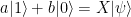
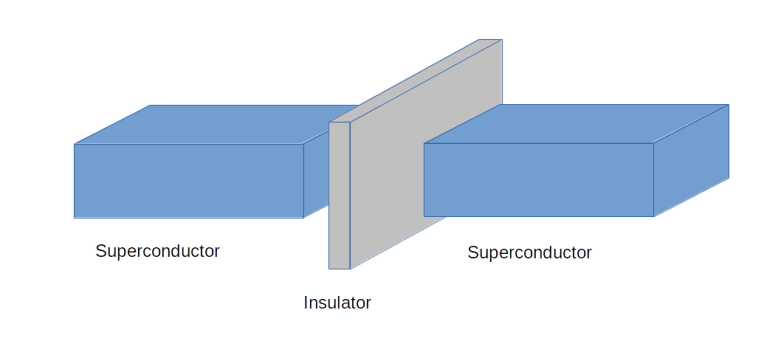
Let us now turn to the real topic of this post – quantum teleportation. Suppose that Alice is in possession of a qubit that captures some quantum state $|\psi \rangle = a |0 \rangle + b|1 \rangle$ , stored in some sort of quantum device, which could be a superconducting qubit, a trapped ion, a polarized photon or any other physical implementation of a qubit. Bob is operating a similar device. The task is to create a quantum state in Bob’s device which is identical to the state stored in Alice device.

To be able to do this, Alice and Bob will need some communication channel. Let us suppose that there is a classical channel that Alice can use to transmit a finite number of bits to Bob. Is that sufficient to transmit the state of the qubit?

Obviously, the answer is no. Alice will not be able to measure both coefficients a and b, and even if she would find a way to do this, she would be faced with the challenge of transmitting two complex numbers with arbitrary precision using a finite string of bits.

At the other extreme, if Alice and Bob were able to fully entangle their quantum devices, they would probably be able to transmit the state. They could for instance implement a swap gate to move the state from Alice device onto Bob’s device.

So if Alice and Bob are able to perform arbitrary entangled quantum operations on the combined system consisting of Alice qubit and Bob’s qubit, a transmission is possible. But what happens if the devices are separated? It turns out that a transmission is still possible based on the classical channel provided that Alice and Bob had a chance to prepare a common state before Alice prepares $|\psi \rangle$ . In fact, this common state does not depend at all on $|\psi \rangle$ , and at no point during the process, any knowledge of the state $|\psi \rangle$ is needed.

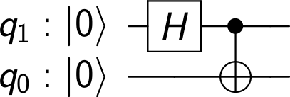
The mechanism first described in [2] works as follows. We need three qubits that we denote by A, B and C. The qubit C contains the unknown state $|\psi \rangle_C$ (we use the lower index to denote the qubit in which the state lives). We also assume that Alice is able to perform arbitrary measurements and operations on A and C, and that B similarly controls qubit B.

The first step in the algorithm is to prepare an entangled state

$|\beta_{00}^{AB} \rangle = \frac{1}{\sqrt{2}} \big[ |0\rangle _A |0 \rangle _B+ |1\rangle_A |1 \rangle_B) \big]$

Here the upper index at $\beta$ indicates the two qubits in which the Bell state vector lives. This is the common state mentioned above, and it can obviously be prepared upfront, without having the state $|\psi \rangle_C$ . Bob and Alice could even prepare an entire repository of such states, ready for being used when the actual transmission should take place.

Now let us look at the state of the combined system consisting of all three qubits.

$|\beta_{00}^{AB} \rangle |\psi\rangle_C = \frac{1}{\sqrt{2}} \big[ a |000 \rangle + a |110 \rangle + b |001\rangle + b |111 \rangle \big]$

For a reason that will become clear in a second, we will now adapt the tensor product order and choose the new order A-C-B. Then our state is (simply swap the last two qubits)

$\frac{1}{\sqrt{2}} \big[ a |000 \rangle + a |101 \rangle + b |010\rangle + b |111 \rangle \big]$

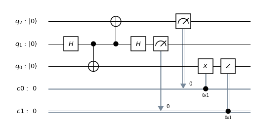
Now instead of using the computational basis for our three-qubit system, we could as well use the basis that is given by the Bell basis of the qubits A and C and the computational basis of B, i.e. $|\beta^{AC}_{ij} \rangle |k\rangle$ . Using the table above, we can express our state in this basis. This will give us four terms that contain a and four terms that contain b. The terms that contain a are

$\frac{a}{2} \big[ |\beta^{AC}_{00}\rangle |0 \rangle + |\beta^{AC}_{10}\rangle |0 \rangle + |\beta^{AC}_{01}\rangle |1 \rangle - |\beta^{AC}_{11} \rangle |1 \rangle \big]$

and the terms that contain b are

$\frac{b}{2} \big[ |\beta^{AC}_{01}\rangle |0 \rangle + |\beta^{AC}_{11}\rangle |0 \rangle + |\beta^{AC}_{00}\rangle |1 \rangle - |\beta^{AC}_{10} \rangle |1 \rangle \big]$

So far we have not done anything to our state, we have simply re-written the state as an expansion into a different basis. Now Alice conducts a measurement – but she measures A and C in the Bell basis. This will project the state onto one of the basis vectors $|\beta_{ij}^{AC}\rangle$ . Thus there are four different possible outcomes of this measurement, which we can read off from the expansion in terms of the Bell basis above.

Measurement	State of qubit B
$\beta_{00}$	$a\|0\rangle + b\|1\rangle = \|\psi \rangle$
$\beta_{01}$	$a\|1\rangle + b\|0\rangle = X\|\psi \rangle$
$\beta_{10}$	$a\|0\rangle - b\|1\rangle = Z\|\psi \rangle$
$\beta_{11}$	$b\|0\rangle - a\|1\rangle = -XZ\|\psi \rangle$

Now Alice sends the outcome of the measurement to Bob using the classical channel. The table above shows that the state in Bob’s qubit B is now the result of a unitary transformation which depends only on the measurement outcome. Thus if Bob receives the measurement outcomes (two bits), he can do a lookup on the table above and apply the inverse transformation on his qubit. If, for instance, he receives the measurement outcome 01, he can apply a Pauli X gate to his qubit and then knows that the state in this qubit will be identical to the original state $|\psi \rangle$ . The teleportation process is complete.

Implementing teleportation as a circuit

Let us now build a circuit that models the teleportation procedure. The first part that we need is a circuit that creates a Bell state (or, more generally, transforms the elements of the computational basis into the Bell basis). This is achieved by the circuit below (which again uses the Qiskit convention that the most significant qubit q₁ is the leftmost one in the tensor product).

It is obvious how this circuit can be reversed – as both individual gates used are there own inverse, we simply need to reverse their order to obtain a circuit that maps the Bell basis to the computational basis.

Let us now see how the overall teleportation circuit looks like. Here is the circuit (drawn with Qiskit).

Let us see how this relates to the above description. First, the role of the qubits is, from the top to the bottom

C = q[2]
A = q[1]
B = q[0]

The first two gates (the Hadamard and the CNOT gate) act on qubits A and B and create the Bell basis vector $\beta_{00}$ from the initial state. This state is the shared entangled state that Alice and Bob prepare upfront.

The next section of the circuit operates on the qubits A and C and realizes the measurement in the Bell basis. We first use a combination of another CNOT gate and another Hadamard gate to map the Bell basis to the computational basis and then perform a measurement – these steps are equivalent to doing a measurement in the Bell basis directly.

Finally, we have a controlled X gate and a controlled Z gate. As described above, these gates apply the conditional corrections to Bob’s state in qubit B that depend on the outcome of the measurement. As a result, the state of qubit B will be the same as the initial state of qubit C.

How can we test this circuit? One approach could be to add a pre-processing part and a post-processing part to our teleportation circuit. The pre-processing gate acts with one or more gates on qubit C to put this qubit into a defined state. We then apply the teleportation circuit. Finally, we apply a post-processing circuit, namely the inverse sequence of gates to the “target” of the teleportation, i.e. to qubit B. If the teleportation works, the pre- and post-steps act on the same logical state and therefore cancel each other. Thus the final result in qubit B will be the initial state of qubit C, i.e. $|0 \rangle$ . Therefore, a measurement of this qubit will always yield zero. Thus our final test circuit looks as follows.

When we run this on a simulator, the result will be as expected – the value in the classical register c2 after the measurement will always be zero. I have not been able to test this on real hardware as the IBM device does not (yet?) support classical conditional gates, but the result is predictable – we would probably get the same output with some noise. If you want to play with the circuits yourself, you can, as always, find the code in my GitHub repository.

So this is quantum teleportation – not quite as mysterious as the name suggests. In particular, we do not magically teleport particles and actual matter, but simply quantum information, based on a clever split of the information contained in an unknown state into a classical part, transmitted in two classical bit, and a quantum part that we can prepare upfront. We also do not violate special relativity – to complete the process, we depend on the measurement outcomes that are transmitted via a classical channel and therefore not faster than the speed of light. It is also important to note that quantum teleportation does also not violate the “no-cloning”-principle – the measurements let the original state collapse and therefore we do not end up with two copies of the same state.

Quantum teleportation has already been demonstrated in reality several times. The first experimental verification was published in [3] in 1997. Since then, the distance between the involved parties “Alice” and “Bob” has been gradually increased. In 2017, a chinese team reported a teleportation of a single qubit between a ground observatory to a low-Earth-orbit satellite (see [4]).

The term quantum teleportation is also used in the context of quantum error correction for a circuit that uses a measurement on an entangled state to bring one of the involved qubits into a specific state. When using a surface code, for instance, this technique – also called gate teleportation – is used to implement the T gate on the level of logical qubits. We refer to [5] for a more detailed discussion of this pattern.

References

1. M. Nielsen, I. Chuang, Quantum Computation and Quantum Information, Cambridge University Press, Cambridge 2010
2. C.H. Bennett, G. Brassard, C. Crepeau, R. Jozsa, A Peres, W.K. Wootter, Teleporting an Unknown Quantum State via Dual Classical and EPR Channels, Phys. Rev. Lett. 70, March 1993
3. D. Bouwmeester, Jian-Wei Pan, K. Mattle, M. Eibl, H. Weinfurter, A. Zeilinger, Experimental quantum teleportation, Nature Vol. 390, Dec. 1997
4. Ji-Gang Ren et. al., Ground-to-satellite quantum teleportation, Nature Vol. 549, September 2017
5. D. Gottesman, I. L. Chuang, Quantum Teleportation is a Universal Computational Primitive, arXiv:quant-ph/9908010

Watching Kubernetes networking in action

In this post, we will look in some more detail into networking in a Kubernetes cluster. Even though the Kubernetes networking model is independent of the underlying cloud provider, the actual implementation does of course depend on the cloud provider which communicates with Kubernetes through a CNI plugin.

I will continue to use EKS, so some of this will be EKS specific. To work with me through the example, you will first have to bring up your cluster, start two nodes and deploy a pod running a httpd on one of the nodes. I have written a script up.sh and a manifest file that automates all this. To download and apply all this, enter

$ git clone https://github.com/christianb93/Kubernetes.git
$ cd Kubernetes/cluster
$ chmod 700 up.sh
$ ./up.sh
$ kubectl apply -f ../pods/alpine.yaml

Node-to-Pod networking

Now let us log into the node on which the container is running and collect some information on the local network interface attached to the VM.

$ ifconfig eth0
eth0: flags=4163  mtu 9001
        inet 192.168.118.64  netmask 255.255.192.0  broadcast 192.168.127.255
        inet6 fe80::2b:dcff:fee7:448c  prefixlen 64  scopeid 0x20
        ether 02:2b:dc:e7:44:8c  txqueuelen 1000  (Ethernet)
        RX packets 197837  bytes 274587781 (261.8 MiB)
        RX errors 0  dropped 0  overruns 0  frame 0
        TX packets 25656  bytes 2389608 (2.2 MiB)
        TX errors 0  dropped 0 overruns 0  carrier 0  collisions 0

So the local IP address of the node is 192.168.118.64. If we do a kubectl get pods -o wide, we get a different IP address – 192.168.99.199 – for the pod. Let us curl this from the node.

$ curl 192.168.99.199
<h1>It works!</h1>

So apparently we have reached our httpd. To understand why this works, let us investigate the network configuration in more detail. First, on the node on which the container is running, let us take a look at the network configuration inside the container.

$ ID=$(docker ps --filter name=alpine-ctr --format "{{.ID}}")
$ docker exec -it $ID "/bin/bash"
bash-4.4# ip link
1: lo:  mtu 65536 qdisc noqueue state UNKNOWN qlen 1000
    link/loopback 00:00:00:00:00:00 brd 00:00:00:00:00:00
3: eth0@if6:  mtu 9001 qdisc noqueue state UP 
    link/ether 4a:8b:c9:bb:8c:8e brd ff:ff:ff:ff:ff:ff
bash-4.4# ifconfig eth0
eth0      Link encap:Ethernet  HWaddr 4A:8B:C9:BB:8C:8E  
          inet addr:192.168.99.199  Bcast:192.168.99.199  Mask:255.255.255.255
          UP BROADCAST RUNNING MULTICAST  MTU:9001  Metric:1
          RX packets:12 errors:0 dropped:0 overruns:0 frame:0
          TX packets:0 errors:0 dropped:0 overruns:0 carrier:0
          collisions:0 txqueuelen:0 
          RX bytes:936 (936.0 B)  TX bytes:0 (0.0 B)
bash-4.4# ip route
default via 169.254.1.1 dev eth0 
169.254.1.1 dev eth0 scope link

What do we learn from this? First, we see that inside the container namespace, there is a virtual ethernet device eth0, with IP address 192.168.99.199. If you run kubectl get pods -o wide on your local workstation, you will find that this is the IP address of the Pod. We also see that there is a route in the container namespace that direct all traffic to this interface. The output of the ip link command also shows that this device is a virtual ethernet device that has a paired device (with index if6) in a different namespace. So let us exit the container, go back to the node and try to figure out what the network configuration on the node is.

$ ip link
1: lo:  mtu 65536 qdisc noqueue state UNKNOWN mode DEFAULT group default qlen 1000
    link/loopback 00:00:00:00:00:00 brd 00:00:00:00:00:00
2: eth0:  mtu 9001 qdisc pfifo_fast state UP mode DEFAULT group default qlen 1000
    link/ether 02:2b:dc:e7:44:8c brd ff:ff:ff:ff:ff:ff
3: eni3f5399ec799:  mtu 9001 qdisc noqueue state UP mode DEFAULT group default 
    link/ether 66:37:e5:82:b1:f6 brd ff:ff:ff:ff:ff:ff link-netnsid 0
4: enie68014839ee@if3:  mtu 9001 qdisc noqueue state UP mode DEFAULT group default 
    link/ether f6:4f:62:dc:38:18 brd ff:ff:ff:ff:ff:ff link-netnsid 1
5: eth1:  mtu 9001 qdisc pfifo_fast state UP mode DEFAULT group default qlen 1000
    link/ether 02:e8:f0:26:a7:3e brd ff:ff:ff:ff:ff:ff
6: eni97d5e6c4397@if3:  mtu 9001 qdisc noqueue state UP mode DEFAULT group default 
    link/ether b2:c9:58:c0:20:25 brd ff:ff:ff:ff:ff:ff link-netnsid 2
$ ifconfig eth0
eth0: flags=4163  mtu 9001
        inet 192.168.118.64  netmask 255.255.192.0  broadcast 192.168.127.255
        inet6 fe80::2b:dcff:fee7:448c  prefixlen 64  scopeid 0x20
        ether 02:2b:dc:e7:44:8c  txqueuelen 1000  (Ethernet)
        RX packets 197837  bytes 274587781 (261.8 MiB)
        RX errors 0  dropped 0  overruns 0  frame 0
        TX packets 25656  bytes 2389608 (2.2 MiB)
        TX errors 0  dropped 0 overruns 0  carrier 0  collisions 0
$ ip route
default via 192.168.64.1 dev eth0 
169.254.169.254 dev eth0 
192.168.64.0/18 dev eth0 proto kernel scope link src 192.168.118.64 
192.168.89.17 dev eni3f5399ec799 scope link 
192.168.99.199 dev eni97d5e6c4397 scope link 
192.168.109.216 dev enie68014839ee scope link

Here we see that – in addition to a few other interfaces – there is a device eth0 to which all traffic is sent by default. However, there is also a device eni97d5e6c4397 which is the other end of the interface visible in the container. And there is a route that sends all traffic that is directed to the IP address of the pod to this interface. Overall, this gives a picture which seems familiar from our earlier analysis of docker networking

If we try to establish a connection to the httpd running in the pod, the routing table entry on the node will send the traffic to the interface eni97d5e6c4397. This is one end of a veth-pair, the other end appears inside the container as eth0. So from the containers point of view, this is incoming traffic received via eth0, which is happily accepted and processed by the httpd. The reply goes the other way – it is directed to eth0 inside the container, travels via the veth pair and ends up inside the host namespace, coming from eni97d5e6c4397.

Pod-to-Pod networking across nodes

Now let us try something else. Log into the second node – on which the container is not running – and try the curl from there. Surprisingly, this works as well! What we have seen so far does not explain this, so there is probably a piece of magic that we are still missing. To find this, let us use the aws cli to print out the network interfaces attached to the node on which the container is running (the following snippet assumes that you have the extremely helpful tool jq installed on your PC).

$ nodeName=$(kubectl get pods --output json | jq -r ".items[0].spec.nodeName")
$ aws ec2 describe-instances --output json --filters Name=private-dns-name,Values=$nodeName --query "Reservations[0].Instances[0].NetworkInterfaces"
---- SNIP -----
{
        "MacAddress": "02:e8:f0:26:a7:3e",
        "SubnetId": "subnet-06088e09ce07546b9",
        "PrivateDnsName": "ip-192-168-84-108.eu-central-1.compute.internal",
        "VpcId": "vpc-060469b2a294de8bd",
        "Status": "in-use",
        "Ipv6Addresses": [],
        "PrivateIpAddress": "192.168.84.108",
        "Groups": [
            {
                "GroupName": "eks-auto-scaling-group-myCluster-NodeSecurityGroup-1JMH4SX5VRWYS",
                "GroupId": "sg-08163e3b40afba712"
            }
        ],
        "NetworkInterfaceId": "eni-0ed2f1cf4b09cb8be",
        "OwnerId": "979256113747",
        "PrivateIpAddresses": [
            {
                "Primary": true,
                "PrivateDnsName": "ip-192-168-84-108.eu-central-1.compute.internal",
                "PrivateIpAddress": "192.168.84.108"
            },
            {
                "Primary": false,
                "PrivateDnsName": "ip-192-168-72-200.eu-central-1.compute.internal",
                "PrivateIpAddress": "192.168.72.200"
            },
            {
                "Primary": false,
                "PrivateDnsName": "ip-192-168-96-163.eu-central-1.compute.internal",
                "PrivateIpAddress": "192.168.96.163"
            },
            {
                "Primary": false,
                "PrivateDnsName": "ip-192-168-99-199.eu-central-1.compute.internal",
                "PrivateIpAddress": "192.168.99.199"
            }
        ],
---- SNIP ----

I have removed some of the output to keep it readable. We see that AWS has attached several elastic network interfaces (ENI) to our node. An ENI is a virtual network interface that AWS creates and manages for you. Each node can have more than one ENI attached, and each ENI can have a primary and multiple secondary IP addresses.

If you look at the last line of the output, you see that there is a network interface eni-0ed2f1cf4b09cb8be that has, as one of the secondary IP addresses, the IP address 192.168.99.199. This is the IP address of our Pod! Let us now go back to the node and inspect its network configuration once more. You will not find a network interface with this exact name, but you will find a network interface on the node on which the pod is running which has the same MAC address, namely eth1.

$ ifconfig eth1
eth1: flags=4163  mtu 9001
        inet6 fe80::e8:f0ff:fe26:a73e  prefixlen 64  scopeid 0x20
        ether 02:e8:f0:26:a7:3e  txqueuelen 1000  (Ethernet)
        RX packets 224  bytes 6970 (6.8 KiB)
        RX errors 0  dropped 0  overruns 0  frame 0
        TX packets 20  bytes 1730 (1.6 KiB)
        TX errors 0  dropped 0 overruns 0  carrier 0  collisions 0

This is an ordinary VPC interface and visible in the entire VPC under all of its IP addresses. So if we curl our httpd from the second node, the traffic will leave that node via the default interface, be picked up by the VPC, routed to the node on which the pod is running and enter via eth1. As IP forwarding is enabled on this node, the traffic will be routed to the Pod and arrive at the httpd.

This is the missing piece of magic we have been looking for. In fact, for every pod running on a node, EKS will add an additional secondary IP address to an ENI attached to the node (and attach additional ENIs if needed) which will make the Pod IP addressses visible in the entire VPC. This mechanism is nicely described in the documentation of the CNI plugin which EKS uses. So we now have the following picture.

So this allows us to run our httpd in such a way that it can be reached from the entire Pod network (and the entire VPC). Note, however, that it can of course not be reached from the outside world. It is interesting to repeat this experiment with a slighly adapted YAML file that uses the containerPort field:

apiVersion: v1
kind: Pod
metadata:
  name: alpine
  namespace: default
spec:
  containers:
  - name: alpine-ctr
    image: httpd:alpine
    ports: 
      - containerPort: 80

If we remove the old Pod and use this YAML file to create a new pod, we will find that the configuration does not change at all. In particular, running docker ps on the node on which the Pod is scheduled will teach you that this port specification is not the equivalent of the port specification of the docker run port mapping feature – as the Kubernetes API specification states, this field is informational.

Implementation of services

Let us now see how this picture changes if we add a service. First, we will use a service of type ClusterIP, i.e. a service that will make our httpd reachable from within the entire cluster under a common IP address. For that purpose – after deleting our existing pods – let us create a deployment that brings up two instances of the httpd.

$ kubectl apply -f https://raw.githubusercontent.com/christianb93/Kubernetes/master/pods/deployment.yaml

Once the pods are up, you can again use curl to verify that you can talk to every pod from every node and every pod. Now let us create a service.

$ kubectl apply -f https://raw.githubusercontent.com/christianb93/Kubernetes/master/network/service.yaml

Once that has been done, enter kubectl get svc to get a list all services. You should see a newly created service alpine-service. Note down its cluster IP address – in my case this was 10.100.11.202.

Now log into one of the nodes again, attach to the container, install curl there and try to connect to port 10.100.11.202:8080

$ ID=$(docker ps --filter name=alpine-ctr --format "{{.ID}}")
$ docker exec -it $ID "/bin/bash"
bash-4.4# apk add curl
OK: 124 MiB in 67 packages
bash-4.4# curl 10.100.11.202:8080
<h1>It works!</h1>

So, as promised by the definition of s service, the httpd is visible within the cluster under the cluster IP address of the service. The same works if we are on a node and not attached to a container.

To see how this works, let us log out of the container again and search the NAT tables for the cluster IP address of the service.

$ sudo iptables -S -t nat | grep 10.100.11.202
-A KUBE-SERVICES -d 10.100.11.202/32 -p tcp -m comment --comment "default/alpine-service: cluster IP" -m tcp --dport 8080 -j KUBE-SVC-SXWLG3AINIW24QJC

So we see that Kubernetes (more precisely the kube-proxy running on each node) has added a NAT rule that captures traffic directed towards the service IP address to a special chain. Let us dump this chain.

$ sudo iptables -S -t nat | grep KUBE-SVC-SXWLG3AINIW24QJC
-N KUBE-SVC-SXWLG3AINIW24QJC
-A KUBE-SERVICES -d 10.100.11.202/32 -p tcp -m comment --comment "default/alpine-service: cluster IP" -m tcp --dport 8080 -j KUBE-SVC-SXWLG3AINIW24QJC
-A KUBE-SVC-SXWLG3AINIW24QJC -m comment --comment "default/alpine-service:" -m statistic --mode random --probability 0.50000000000 -j KUBE-SEP-YRELRNVKKL7AIZL7
-A KUBE-SVC-SXWLG3AINIW24QJC -m comment --comment "default/alpine-service:" -j KUBE-SEP-BSEIKPIPEEZDAU6E

Now this is actually pretty interesting. The first line is simply the creation of the chain. The second line is the line that we already looked at above. The next two lines are the lines we are looking for. We see that, with a probability of 50%, we either jump to the chain KUBE-SEP-YRELRNVKKL7AIZL7 or to the chain KUBE-SEP-BSEIKPIPEEZDAU6E. Let us display one of them.

$ sudo iptables -S KUBE-SEP-BSEIKPIPEEZDAU6E -t nat 
-N KUBE-SEP-BSEIKPIPEEZDAU6E
-A KUBE-SEP-BSEIKPIPEEZDAU6E -s 192.168.191.152/32 -m comment --comment "default/alpine-service:" -j KUBE-MARK-MASQ
-A KUBE-SEP-BSEIKPIPEEZDAU6E -p tcp -m comment --comment "default/alpine-service:" -m tcp -j DNAT --to-destination 192.168.191.152:80

So we see the that this chain has two rules. The first rule marks all packages that are originating from the pod running on this node, this mark is later evaluated in the forwarding rules to make sure that the packet is accepted for forwarding. The second rule is where the magic happens – it performs a DNAT, i.e. a destination NAT, and sends our packets to one of the pods. The rule KUBE-SEP-YRELRNVKKL7AIZL7 is similar, with the only difference that it sends the packets to the other pod. So we see that two things are happening

Traffic directed towards port 8080 of the cluster IP address is diverted to one of the pods
Which one of the pods is selected is determined randomly, with a probability of 50% for both pods. Thus these rules implement a simple load balancer.

Let us now see how things change when we use a service of type NodePort. So let us use a slightly different YAML file.

$ kubectl delete -f https://raw.githubusercontent.com/christianb93/Kubernetes/master/network/service.yaml
$ kubectl apply -f https://raw.githubusercontent.com/christianb93/Kubernetes/master/network/nodePortService.yaml

When we now run kubectl get svc, we see that our service appears as a NodePort service, and, as the second entry in the columns PORTS, we find the port that Kubernetes opens for us.

$ kubectl get services
NAME             TYPE        CLUSTER-IP     EXTERNAL-IP   PORT(S)          AGE
alpine-service   NodePort    10.100.165.3           8080:32755/TCP   13s
kubernetes       ClusterIP   10.100.0.1             443/TCP          7h

In my case, the port 32755 has been used. If we now go back to one of the nodes and search the iptables rules for this port, we find that Kubernetes has created two additional NAT rules.

$ sudo iptables -S  -t nat | grep 32755
-A KUBE-NODEPORTS -p tcp -m comment --comment "default/alpine-service:" -m tcp --dport 32755 -j KUBE-MARK-MASQ
-A KUBE-NODEPORTS -p tcp -m comment --comment "default/alpine-service:" -m tcp --dport 32755 -j KUBE-SVC-SXWLG3AINIW24QJC

So we find that for all traffic directed to this port, again a marker is set and the rule KUBE-SVC-SXWLG3AINIW24QJC applies. If you inspect this rule, you will find that it is similar to the rules above and again realizes a load balancer that sends traffic to port 80 of one of the pods.

Let us now verify that we can really reach this pod from the outside world. Of course, this only works once we have allowed incoming traffic on at least one of the nodes in the respective AWS security group. The following commands determine the node Port, your IP address, the security group and the IP address of the node, allow access and submit the curl command (note that I use the cluster name myCluster to select the worker nodes, in case you are not using my scripts to run this example, you will have to change the filter to make this work).

$ nodePort=$(kubectl get svc alpine-service --output json | jq ".spec.ports[0].nodePort")
$ IP=$(aws ec2 describe-instances --filters Name=tag-key,Values=kubernetes.io/cluster/myCluster Name=instance-state-name,Values=running --output text --query Reservations[0].Instances[0].PublicIpAddress)
$ SEC_GROUP_ID=$(aws ec2 describe-instances --filters Name=tag-key,Values=kubernetes.io/cluster/myCluster Name=instance-state-name,Values=running --output text --query Reservations[0].Instances[0].SecurityGroups[0].GroupId)
$ myIP=$(wget -q -O- https://ipecho.net/plain)
$ aws ec2 authorize-security-group-ingress --group-id $SEC_GROUP_ID --port $nodePort --protocol tcp --cidr "$myIP/32"
$ curl $IP:$nodePort
<h1>It works!</h1>

Summary

After all these nitty-gritty details, let us summarize what we have found. When you start a pod on a node, a pair of virtual ethernet devices is created, with one end being assigned to the namespace of the container and one end being assigned to the namespace of the host. Then IP routes are added so that traffic directed towards the pod is forwarded to this bridge. This allows access to the container from the node on which they are running. To realize access from other nodes and pods and thus the flat Kubernetes networking model, EKS uses the AWS CNI plugin which attaches the pods IP addresses as secondary IP addresses to elastic network interfaces.

When you start a service, Kubernetes will in addition set up NAT rules that will capture traffic determined for the cluster IP address of the service and perform a destination network address translation so that this traffic gets send to one of the pods. The pod is selected at random, which implements a simple load balancer. For a service of type NodePort, additional rules will be created which make sure that the same NAT processing applies to traffic coming from the outside world.

This completes today post. If you want to learn more, you might want to check out some of the links below.

this post by Kevin Sookocheff
the source code of the iptable interface of the kube proxy
The proposal for the AWS CNI plugin
my own series on networking in Docker (part I, part II)
and of course the Kubernetes documention itself

Computational basis vector	Bell basis vector
$\|00 \rangle$	$\|\beta_{00} \rangle = \frac{1}{\sqrt{2}} (\|00 \rangle + \|11 \rangle)$
$\|01 \rangle$	$\|\beta_{01} \rangle = \frac{1}{\sqrt{2}} (\|01 \rangle + \|10 \rangle)$
$\|10 \rangle$	$\|\beta_{10} \rangle = \frac{1}{\sqrt{2}} (\|00 \rangle - \|11 \rangle)$
$\|11 \rangle$	$\|\beta_{11} \rangle = \frac{1}{\sqrt{2}} (\|01 \rangle - \|10 \rangle)$