Python – Page 6 – LeftAsExercise

Setting up and testing our bitcoin network

In the last post in my series on bitcoin and the blockchain, we have successfully “dockerized” the bitcoin core reference implementation and have built the bitcoin-alpine docker container that contains a bitcoin server node on top of the Alpine Linux distribution. In this post, we will use this container image to build up and initialize a small network with three nodes.

First, we start a node that will represent the user Alice and manage her wallet.

$ docker run -it --name="alice" -h="alice" bitcoin-alpine

Note that we have started the container with the option -it so that it stays attached to the current terminal and we can see its output. Let us call this terminal terminal 1. We can now open a second terminal and attach to the running server and use the bitcoin CLI to verify that our server is running properly.

$ docker exec -it alice  "sh"
# bitcoin-cli -regtest --rpcuser=user --rpcpassword=password getinfo

If you run – as shown above – the bitcoin CLI inside the container using the getbalance RPC call, you will find that at this point, the balance is still zero. This not surprising, our network does not contain any bitcoins yet. To create bitcoins, we will now bring up a miner node and mine a certain amount of bitcoin. So in a third terminal, enter

$ docker run -it --name="miner" -h="miner" bitcoin-alpine

This will create a second node called miner and start a second instance of the bitcoin server within this network. Now, however, our two nodes are not yet connected. To change this, we can use the addnode command in the bitcoin CLI. So let us figure out how they can reach each other on the network. We have started both containers without any explicit networking options, so they will be connected to the default bridge network that Docker creates on your host. To figure out the IP addresses, run

$ docker network inspect bridge

on your host. This should produce a list of network devices in JSON format and spit out the IP addresses of the two nodes. In my case, the node alice has the IP address 172.17.0.2 and the miner has the IP address 172.17.0.3. So let us change back to terminal number 2 (attached to the container alice) and run

# bitcoin-cli -regtest --rpcuser=user --rpcpassword=password addnode 172.17.0.3 add

In the two terminal windows that are displaying the output of the two bitcoin daemons on the nodes alice and miner, you should now see an output similar to the following.

2018-03-24 14:45:38 receive version message: /Satoshi:0.15.0/: version 70015, blocks=0, us=[::]:0, peer=0

This tells you that the two peers have exchanged a version message and recognized each other. Now let us mine a few bitcoins. First attach a terminal to the miner node – this will be terminal four.

$ docker exec -it miner "sh"

In that shell, enter the following command

# bitcoin-cli -regtest --rpcuser=user --rpcpassword=password generate 101
# bitcoin-cli -regtest --rpcuser=user --rpcpassword=password getbalance

You should now see a balance of 50 bitcoins. So we have mined 50 bitcoins (in fact, we have mined much more, but it requires additional 100 blocks before a mined transaction is considered to be part of the balance and therefore only the amount of 50 bitcoins corresponding to the very first block shows up).

This is already nice, but when you execute the RPC method getbalance in terminal two, you will still find that Alice balance is zero – which is not surprising, after all the bitcoins created so far have been credited to the miner, not to Alice. To change this, we will now transfer 30 bitcoin to Alice. As a first step, we need to figure out what Alice address is. Each wallet maintains a default account, but we can add as many accounts as we like. So let us now add an account called “Alice” on the alice node. Execute the following command in terminal two which is attached to the container alice.

# bitcoin-cli -regtest --rpcuser=user --rpcpassword=password getnewaddress "Alice"

The output should be something like mkvAYmgqrEFEsJ9zGBi9Z87gP5rGNAu2mx which is the bitcoin address that the wallet has created. Of course you will get a different address, as the private key behind that address will be chosen randomly by the wallet. Now switch to the terminal attached to the miner node (terminal four). We will now transfer 30 bitcoin from this node to the newly created address of Alice.

# bitcoin-cli -regtest --rpcuser=user --rpcpassword=password sendtoaddress "mkvAYmgqrEFEsJ9zGBi9Z87gP5rGNAu2mx" 30.0

The output will be the transaction ID of the newly created transaction, in my case this was

2bade389ac5b3feabcdd898b8e437c1d464987b6ac1170a06fcb24ecb24986a8

If you now display the balances on both nodes again, you will see that the balance in the default account on the miner node has dropped to something a bit below 20 (not exactly 20, because the wallet has added a fee to the transaction). The balance of Alice, however, is still zero. The reason is that the transaction does not yet count as confirmed. To confirm it, we need to mine six additional blocks. So let us switch to the miners terminal once more and enter

# bitcoin-cli -regtest --rpcuser=user --rpcpassword=password generate 6

If you now display the balance on the node alice, you should find that the balance is now 30.

Congratulations – our setup is complete, we have run our first transaction and now have plenty of bitcoin in a known address that we can use. To preserve this wonderful state of the world, we will now create two new images that contain snapshots of the nodes so that we have a clearly defined state to which we can always return when we run some tests and mess up our test data. So switch back to a terminal on your host and enter the following four commands.

$ docker stop miner
$ docker stop alice
$ docker commit miner miner
$ docker commit alice alice

If you now list the available images using docker images, you should see two new images alice and miner. If you want, you can now remove the stopped container instances using docker rm.

Now let us see how we can talk to a running server in Python. For that purpose, let us start a detached container using our brand new alice image.

$ docker run  -d --rm --name=alice -p 18332:18332 alice

We can now communicate with the server using RPC requests. The bitcoin RPC interface follows the JSON RPC standard. Using the powerful Python package requests, it is not difficult to write a short function that submits a request and interprets the result.

def rpcCall(method, params = None, port=18332, host="localhost", user="user", password="password"):
    #
    # Create request header
    #
    headers = {'content-type': 'application/json'}
    #
    # Build URL from host and port information
    #
    url = "http://" + host + ":" + str(port)
    #
    # Assemble payload as a Python dictionary
    # 
    payload = {"method": method, "params": params, "jsonrpc": "2.0", "id": 1}        
    #
    # Create and send POST request
    #
    r = requests.post(url, json=payload, headers=headers, auth=(user, password))
    #
    # and interpret result
    #
    json = r.json()
    if 'result' in json and json['result'] != None:
        return json['result']
    elif 'error' in json:
        raise ConnectionError("Request failed with RPC error", json['error'])
    else:
        raise ConnectionError("Request failed with HTTP status code ", r.status_code)

If have added this function to my btc bitcoin library within the module utils. We can use this function in a Python program or an interactive ipython session similar to the bitcoin CLI client. The following ipython session demonstrates a few calls, assuming that you have cloned the repository.

In [1]: import btc.utils
In [2]: r = btc.utils.rpcCall("listaccounts")
In [3]: r
Out[3]: {'': 0.0, 'Alice': 30.0}
In [4]: r = btc.utils.rpcCall("dumpprivkey", ["mkvAYmgqrEFEsJ9zGBi9Z87gP5rGNAu2mx"])
In [5]: r
Out[5]: 'cQowgjRpUocje98dhJrondLbHNmgJgAFKdUJjCTtd3VeMfWeaHh7'

We are now able to start our test network at any time from the saved docker images and communicate with it using RPC calls in Python. In the next post, we will see how a transaction is created, signed and propagated into the test network.

Learning algorithms for restricted Boltzmann machines – contrastive divergence

In the previous post on RBMs, we have derived the following gradient descent update rule for the weights.

$\Delta W_{ij} = \beta \left[ \langle v_i \sigma(\beta a_j) \rangle_{\mathcal D} - \langle v_i \sigma(\beta a_j) \rangle_{P(v)} \right]$

In this post, we will see how this update rule can be efficiently implemented. The first thing that we note is that the term $\sigma(\beta a_j)$ that appears several times is simply the conditional probability for the hidden unit j to be “on” and, as only the values 0 and 1 are possible, at the same time the conditional expectation value of that unit given the values of the visible units – let us denote this quantity by $e_j$ . Our update rule now reads

$\Delta W_{ij} = \beta \left[ \langle v_i e_j \rangle_{\mathcal D} - \langle v_i e_j \rangle_{P(v)} \right]$

Theoretically, we know how to calculate this. The first term – the positive phase – is easy, this is just the average over the sample set.

The second term is more challenging. Theoretically, we would need a Gibbs sampler to calculate it using a Monte Carlo approach. One step of this sampler would proceed as follows.

Given the values v of the visible units, calculate the resulting expectation values e
Set hidden unit j to one with probability e_j
For each visible unit i, calculate the conditional probability p_i to be one given the new values of the hidden units
Set v_i to 1 with probability p_i

After some burn-in phase, we would then calculate the product $v_i e_j$ after each step and take the average of these values.

The crucial point is that for a naive implementation, we would start the Gibbs sampling procedure during each gradient descent iteration from scratch, i.e. with some randomly initialized values for the visible units. One of the ideas behind the algorithm known as contrastive divergence that was proposed by G. Hinton in [1] is to restart the Gibbs sampler not at a random value, but a randomly chosen vector from the data set! The idea behind this is that if we have been running the training for some time, the model distribution should be close to the empirical distribution of the data, so sampling a vector from the data should give us something close to the equilibrium state of the Gibbs sampling Markov chain (if you do not known what a Markov chain is – do not worry and just read on, I will cover Markov chains and the mathematics behind all this in a later post).

The second approximation that the contrastive divergence algorithm makes is to replace the expectation values in the positive and negative phase by a point estimate. For the positive phase, that means we simply calculate the value at one point from the data set. For the negative phase, we run the Gibbs sampling procedure – starting as explained above with a vector from the data set – and then simply compute the product $v_i e_j$ for the result.

It now turns out that, based on empirical observations, these approximations work extremely well – in fact, it turns out that instead of running a full Gibbs sampler with a few hundred or even a few thousand steps, one step is often sufficient! This is surprising, but open to an intuitive explanation – we run all this within the outer loop provided by the gradient descent algorithm, and if we chose the learning rate sufficiently small, the parameters do not change a lot between these steps, so that we effectively do something that is close to one long Gibbs sampling Markov chain.

With these simplifications, the constrastive divergence algorithm now looks as follows.

FOR EACH iteration DO

Sample a vector v from the data set

SET $e = \sigma(\beta( W^T v + c))$

FOR EACH hidden unit DO

SET $h_j = 1$ with probability $e_j$

FOR EACH visible unit DO

SET $\bar{v}_i = 1$ with probability $\sigma(\beta (W h + b))_i$

SET $\bar{e} = \sigma(\beta (W^T \bar{v} + c))$

SET $W = W + \lambda \beta \left[ v e^T - \bar{v} \bar{e}^T \right]$

SET $b = b + \lambda \beta \left[ v - \bar{v} \right]$

SET $c = c + \lambda \beta \left[ e - \bar{e} \right]$

DONE

The first six lines within an iteration constitute one Gibbs sampling step, starting with a value for the visible units from the data set, sampling the hidden units from the visible units and sampling the visible units from the hidden units. In the next line, we recalculate the expectation values of the hidden units given the (updated) values of the visible units. The value $\bar{v}_i \bar{e}_j$ is then the contribution of the negative phase to the update of $W_{ij}$ . We can summarize the contributions for all pairs of indices as the matrix $\bar{v} \bar{e}^T$ . Similarly, the positive phase contributes with $v e^T$ . In the next line, we update W with both contributions, where $\lambda$ is the learning rate. We then apply similar update rules to the bias for visible and hidden units – the derivation of these update rules from the expression for the likelihood function is done similar to the derivation of the update rules for the weights as shown in my last post.

Let us now implement this in Python. To have a small data set for our tests, we will use an artificial data set called bars and stripes that I have seen first in [3]. Given a number N, we can create an image with N x N pixels for every number x smallers than 2^N as follows. Each row corresponds to one binary digit of x. If this digit is one, the entire row is black, i.e. we have one black vertical stripe, otherwise the entire row is white. A second row of patterns is obtained by coloring the columns similarly instead of the rows. Thus we obtain 2^N+1 possible patterns, more than enough for our purposes. I have written a helper class BAS in Python that creates these patterns.

Next, let us turn to the actual RBM. We store the current state of the RBM in a class RBM that is initialized as follows.

class RBM:

    def __init__ (self, visible = 8, hidden = 3, beta = 1):
        self.visible = visible
        self.hidden = hidden
        self.beta = beta
        self.W = np.random.normal(loc = 0, scale = 0.01, size = (visible, hidden))
        self.b = np.zeros(shape = (1,visible))
        self.c = np.zeros(shape = (1,hidden))

Here W is the weight matrix, beta is the inverse temperature, and b and c are the bias vectors for the visible and hidden units.

Next we need a method that runs one step in a Gibbs sampling chain, starting with a state of the visible units captured in a matrix V (we calculate this in a mini-batch for more than one sample at a time, each row in the matrix represents one sample vector). Using once more the numpy library, this can be done as follows.

def runGibbsStep(self, V, size = 1):
    #
    # Sample hidden units from visible units
    #
    E = expit(self.beta*(np.matmul(V, self.W) + self.c))
    U = np.random.random_sample(size=(size, self.hidden))
    H = (U <= E).astype(int)
    #
    # and now sample visible units from hidden units
    #
    P = expit(self.beta*(np.matmul(H, np.transpose(self.W)) + self.b))
    U = np.random.random_sample(size=(size, self.visible))
    return (U <= P).astype(int), E

With this method at hand – which returns the new value for the visible units but the old value for the conditional expectation of the hidden units – we can now code our training routine.

def train(self,  V, iterations = 100, step = 0.01):
    batch_size = V.shape[0]
    #
    # Do the actual training. First we calculate the expectation
    # values of the hidden units given the visible units. The result
    # will be a matrix of shape (batch_size, hidden)
    #
    for _ in range(iterations):
        #
        # Run one Gibbs sampling step and obtain new values
        # for visible units and previous expectation values
        #
        Vb, E = self.runGibbsStep(V, batch_size)
        #
        # Calculate new expectation values
        #
        Eb = expit(self.beta*(np.matmul(Vb, self.W) + self.c))
        #
        # Calculate contributions of positive and negative phase
        # and update weights and bias
        #
        pos = np.tensordot(V, E, axes=((0),(0)))
        neg = np.tensordot(Vb, Eb, axes=((0),(0)))
        dW = step*self.beta*(pos -neg) / float(batch_size)
        self.W += dW
        self.b += step*self.beta*np.sum(V - Vb, 0) / float(batch_size)
        self.c += step*self.beta*np.sum(E - Eb, 0) / float(batch_size)

Let us now play around with this network a bit and visualize the training results. To do this, clone my repository and then run the simulation using

$ git clone  https://github.com/christianb93/MachineLearning.git
$ cd MachineLearning
$ python RBM.py  --run_reconstructions=1 --show_metrics=1

This will train a restricted Boltzmann machine on 20 images out of the BAS dataset with N=6. For the training, I have used standard parameters (which you can change using the various command line switches, use --help to see which parameters are available). The learning rate was set to 0.05. The number of iterations during training was set to 30.000, and 16 hidden units are used. The inverse temperature $\beta$ is set to 2.0. In each iteration, a mini-batch of 10 patterns is trained.

After every 500 iterations, the script prints out the current value of the reconstruction error. This is defined to be the norm of the difference between the value of the visible units when the Gibbs sampling step starts and the value after completing the Gibbs sampling step, i.e. this quantity measures how well the network is able to reconstruct the value of the visible units from the hidden units alone.

After the training phase is completed, the script will select eight patterns randomly. For each of these patterns, it will flip a few bits and then run 100 Gibbs sampling steps. If the training was successful, we expect that the result will be a reconstruction of the original image, i.e. the network would be able to match the distorted images to the original patterns.

When all the calculations have been completed, the network will display two images. The first image should roughly look like the image below.

This matrix visualizes the result of the reconstruction process described above. Each of the rows shows the outcome for one of the eight selected patterns. The first image in each row is the original pattern from the BAS data set. The second one is the distorted image some pixels have been flipped. The third image shows the result of the reconstruction run after 50 Gibbs iterations, and the last image shows the result after the full 100 iterations.

We see that in most cases, the network is able to correctly reconstruct the original image. However, there are also a fes rows that look suspicious. In the first row, we could hope that the network eventually converges if we execute more sampling steps. In the third row, however, the network converges to a member of the BAS data set, but to the wrong one.

The second diagram that the script produces displays the change to the weights after each iteration and the reconstruction error.

We see that both quantities quickly get smaller, but never stabilize at exactly zero. This is not really surprising – as we work with a non-zero temperature, we will always have some thermal fluctuations and the reconstruction error will never be constantly zero, but oscillate around a small value.

I invite you to play around with the parameters a bit to see how the network behaves. We can change the value of the inverse temperature with the parameter --beta, the number of hidden units with the parameter --hidden, the number of Gibbs steps used during the reconstruction with --sample and the step size with --step. If, for instance, you raise the temperature, the fluctuations of the reconstruction error will increase. If, one the other hand, we choose a very small temperature, the network converges very slowly. Making the step size too small or too large can also lead to non-convergence etc.

That completes this post on contrastive divergence. In the next post, I will show you an alternative algorithm that has gained a lot of popularity called persistent contrastive divergence (PCD), before we finally set out to implement an restricted Boltzmann machine on a GPU using the TensorFlow framework.

1. G. Hinton, Training products of experts by minimizing contrastive divergence, Journal Neural Computation Vol. 14, No. 8 (2002), 1771 1800
2. G. Hinton, A practical guide to training restricted Boltzmann machines, Technical Report University of Montreal TR-2010-003 (2010)
[3] D. MacKay, Information Theory, Inference and learning
algorithms, section 43, available online at this URL

Signing and verifying bitcoin transactions

If you have followed my blockchain posts so far, you know how to create bitcoin transactions by assembling transaction inputs and transaction outputs into a transaction data structure and serializing it. However, there is one subtlety that we have ignored so far – what exactly do you sign?

You cannot sign the entire bitcoin transaction, simply because the signature is part of it! So there is a sort of chicken-or-egg problem. Instead, you need to build a transaction without the signature, serialize it, create a hash value, sign this hash value, then add the signature to the transaction and publish this transaction.

This is essentially how signing actually works. However, there are a few details that we still miss. So let us look at the source code of the reference client once more to make sure that we really understand how this works.

As a starting point, remember that there is a script opcode called OP_CHECKSIG that verifies a signature. So let us look at the corresponding method which we find in script/interpreter.cpp. When this opcode is executed, the function EvalScript delegates to the method TransactionSignatureChecker::CheckSig. This method removes the last byte of the signature script (which is the hash type) and then calls the function SignatureHash. This function receives the following parameters (you might have to trace back a bit starting at EvalScript to verify this):

the script code of the public key script
the transaction that is to be signed
the index of the transaction input within that transaction to which the signature refers
the hash type
the amount
a version number which is zero in our case and indicates whether the segregated witness feature is in effect
a data structure that serves as a cache

We have not yet talked about the hash type. Essentially the hash type controls which parts of a transaction are included in the signature and therefore protected against being changed. The most common case is SIGHASH_ALL = 1, and this is the value for this field that we assume in this post (if you understand this case, it will not be difficult to figure out the other cases as well).

In any case, the function SignatureHash is what we are searching for. It serializes the transaction and creates a hash value which is then passed to the crytographic subroutines to actually verify the signature. This function again delegates the actual work to an instance of the helper class CTransactionSignatureSerializer, more precisely to its method Serialize. This method is in fact not very surprising.

template
void Serialize(S &s) const {
    // Serialize nVersion
    ::Serialize(s, txTo.nVersion);
    // Serialize vin
    unsigned int nInputs = fAnyoneCanPay ? 1 : txTo.vin.size();
    ::WriteCompactSize(s, nInputs);
    for (unsigned int nInput = 0; nInput < nInputs; nInput++)
         SerializeInput(s, nInput);
    // Serialize vout
    unsigned int nOutputs = fHashNone ? 0 : (fHashSingle ? nIn+1 : txTo.vout.size());
    ::WriteCompactSize(s, nOutputs);
    for (unsigned int nOutput = 0; nOutput < nOutputs; nOutput++)
         SerializeOutput(s, nOutput);
    // Serialize nLockTime
    ::Serialize(s, txTo.nLockTime);
}

Ignoring the flag fAnyoneCanPay, this method behaves similar to ordinary serialization – first the version number is written, then the number of inputs, followed by the actual inputs, then the number of outputs, the actual outputs and finally the lock time.

The actual difference to an ordinary transaction serialization is hidden in the method SerializeInput.

template
void SerializeInput(S &s, unsigned int nInput) const {
    // In case of SIGHASH_ANYONECANPAY, only the input being signed is serialized
    if (fAnyoneCanPay)
        nInput = nIn;
    // Serialize the prevout
    ::Serialize(s, txTo.vin[nInput].prevout);
    // Serialize the script
    if (nInput != nIn)
        // Blank out other inputs' signatures
        ::Serialize(s, CScript());
    else
        SerializeScriptCode(s);
    // Serialize the nSequence
    if (nInput != nIn && (fHashSingle || fHashNone))
        // let the others update at will
        ::Serialize(s, (int)0);
    else
        ::Serialize(s, txTo.vin[nInput].nSequence);
}

Again, this starts out as usual by serializing the reference to the spent transaction output (transaction ID and index). However, we soon find the first difference – if the index of the transaction input to be signed differs from the input that is currently serialized, an empty script is serialized instead of the signature script – which translates into a single byte 0x0 which is the length of the empty script.

The second difference is located in the method SerializeScriptCode. Here, instead of serializing the not yet existing signature, the content of the variable scriptCode is serialized. Going back a bit, we see that this is the public key script of the corresponding transaction output! So basically, this script takes the position of the signature script in this serialization step.

But we are not yet done – let us return to the function SignatureHash and see what it does close to the end.

CTransactionSignatureSerializer txTmp(txTo, scriptCode, nIn, nHashType);

// Serialize and hash
CHashWriter ss(SER_GETHASH, 0);
ss << txTmp << nHashType;
return ss.GetHash();

Using the operator <<, we see that the method Serialize that we have just studied is invoked. However, we see that in addition, the hash type – which was stripped off at the beginning – is now added again at the end. All this is routed into a CHashWriter which is defined in hash.h and is essentially a wrapper around a 256 bit hashing routine. This hash is then returned to TransactionSignatureChecker::CheckSig which then tries to verify the signature with that message.

After that tour through the reference client, let us try to verify the signature of a real transaction from the bitcoin network. In the library btc/script.py, I have implemented a function signatureHash which does – for the special case discussed – the same as the function that we have just looked at. Using that function, it is now not difficult to verify a signature, given a transaction input and the corresponding spent output. Here is what we need to do in an ipython session, again assuming that you have downloaded my btc package.

First, we get our sample transaction that we have already used before and the transaction output spent by the first transaction input.

In [1]: import btc.utils
In [2]: import btc.txn
In [3]: raw = btc.utils.getRawTransaction("ed70b8c66a4b064cfe992a097b3406fa81ff09641fe55a709e4266167ef47891")
In [4]: txn = btc.txn.txn()
In [5]: txn.deserialize(raw)
In [6]: txin = txn.getInputs()[0]
In [7]: raw = btc.utils.getRawTransaction(txin.prevTxid)
In [8]: prev = btc.txn.txn()
In [9]: prev.deserialize(raw)
In [10]: spentTxo = prev.getOutputs()[txin.getVout()]

Next, we determine the signature hash and interpret it as a big endian encoded integer.

In [11]: h = int.from_bytes(btc.script.signatureHash(txn, 0, spentTxo), "big")

Next we need to determine the other ingredients of the signature – the r and s values.

In [12]: r = txin.getScriptSig().getSignatureR()
In [13]: s = txin.getScriptSig().getSignatureS()

Now we need the ECDSA cryptography library. We get the SECP256K1 curve and its parameters from there and determine the point on the curve that corresponds to the public key.

In [14]: import ecdsa
In [15]: curve = ecdsa.curves.SECP256k1
In [16]: G = curve.generator
In [17]: p = curve.curve.p()
In [18]: txin.getScriptSig().getScriptType()
Out[18]: 'P2PKH'
In [19]: pubKey = txin.getScriptSig().getPubKeyHex()
In [20]: pubKey
Out[20]: '038c2d1cbe4d731c69e67d16c52682e01cb70b046ead63e90bf793f52f541dafbd'

We see that the first byte of the public key is 0x03. If you remember what we have learned about the public key encoding, this means that y is odd. We can therefore determine the x and y coordinate as follows.

In [21]: x = int.from_bytes(bytes.fromhex(pubKey[2:66]), 'big')
In [22]: y = ecdsa.numbertheory.square_root_mod_prime((x**3 +7) % p , p)
In [23]: y
Out[23]: 91238655223056717466178782248030327689649326505413694215614940048183357985838
In [24]: y = (p - y) % p
In [25]: y
Out[25]: 24553434014259477957392202760657580163620658160226869823842643959725476685825
In [26]: assert(curve.curve.contains_point(x, y))

Now we are almost done.

In [27]: Q = ecdsa.ellipticcurve.Point(curve.curve, x, y)
In [28]: pKey = ecdsa.ecdsa.Public_key(G, Q)
In [29]: signature = ecdsa.ecdsa.Signature(r,s)
In [30]: pKey.verifies(h, signature)
Out[30]: True

So our signature is valid, as expected – after all this is a real transaction from the bitcoin network. The full source code for this exercise is also contained in btc/script.py in the function verifySignature.

Of course we could now revert this process – given a transaction, we could use the function signatureHash to create a hash value which we then sign using the ECDSA library. This now puts us in a position to actually create a transaction that we can then push into the bitcoin network. Now, this is clearly something you do not want to try in the real bitcoin network. Therefore I will show you in my next post how you can set up a small test network at home to be able to play with this without the risk of losing actual bitcoins.

Hopfield networks: practice

After having discussed Hopfield networks from a more theoretical point of view, let us now see how we can implement a Hopfield network in Python.

First let us take a look at the data structures. We will store the weights and the state of the units in a class HopfieldNetwork. The weights are stored in a matrix, the states in an array.

class HopfieldNetwork:

    #
    # Initialize a Hopfield network with N
    # neurons
    #
    def __init__(self, N):
        self.N = N
        self.W = np.zeros((N,N))
        self.s = np.zeros((N,1))

Next we write a method for the update rule. In a matrix notation, the activation of unit i is given as the dot product of the current state and the i-th row of the weight matrix (or the i-th column, as the matrix is symmetric). Therefore we can use the following update function.

#
# Run one simulation step
#
def runStep(self):
    i = np.random.randint(0,self.N)
    a = np.matmul(self.W[i,:], self.s)
    if a < 0:
        self.s[i] = -1
    else:
        self.s[i] = 1

Finally, there is the Hebbian learning rule. If we store the sample set in a matrix S such that each row corresponds to one sample, the learning rule is equivalent to

$W = S^T S$

Thus we can again use the matrix multiplication from the numpy package, and our learning rule is simply

def train(self, S):
    self.W = np.matmul(S.transpose(), S)

Now we need some pattern to train our network. For the sake of demonstration, let us use a small network with 5 x 5 units, each of them representing a pixel in a grayscale 5 x 5 image. For this post, I have hardcoded five simple patterns, but we could of course use any other training set.

To illustrate how the Hopfield network operates, we can now use the method train to train the network on a few of these patterns that we call memories. We then take these memories and randomly flip a few bits in each of them, in other words we simulate random errors in the pattern. We then place the network in these states and run the update rule several times. If you want to try this yourself, get the script Hopfield.py from my GitHub repository.

The image above shows the result of this exercise. Here we have stored three memories – the first column of images – in the network. The second image in each row then shows the distorted versions of these patterns after flipping five bits randomly. The next images in each row show the state of the network after 20, 40, 60, 80 and 100 iterations of the update rule. We see that in this case, all errors could be removed and the network did in fact converge to the original image.

However, the situation becomes worse if we try to store more memories. The next image shows the outcome of a simulation with the same basic parameters, but five instead of three memories.

We clearly see that not a single one of the distorted patterns converges to the original image. Apparently, we have exceeded the capacity of the network. In his paper, Hopfield – based on theoretical considerations and simulations – argues that the network can only store approximately $0.15 \cdot N$ patterns, where N is the number of units. In our case, with 25 units, this would be approximately 3 to 4 patterns.

If we exceed this limit, we seem to create local minima of the energy that do not correspond to any of the stored patterns. This problem is known as the problem of spurious minima which can also occur if we stay below the maximum capacity – if you do several runs with three memories, you will find that also in this case, spurious minima can occur.

The update rule of the Hopfield network is deterministic, its energy can never increase. Thus if the system moves into one of those local minima, it can never escape again and gets stuck. An Ising model at a finite, non-zero temperature behaves differently. As the update rule is stochastic, it is possible that the system moves away from a local minimum in a Gibbs sampling step, and therefore has the chance to escape from a spurious minimum. This is one of the reasons why researchers have tried to come up with stochastic versions of the Hopfield network. One of these stochastic versions is the Boltzmann network, and we will start to look at its theoretical foundations in the next post in this series.

Scripts in the bitcoin protocol

There is a point that we have touched upon several times but not yet properly explained – the role of scripts in the bitcoin protocol. We have seen that the public key and the signature are stored inside a bitcoin transaction in container data structures that were called scriptPubKey and scriptSig in the source code. But scripts are more than just container for data, they are in fact executable and do not only store keys and signatures but also instruct the bitcoin server what to do with this data in order to validate a signature.

So what is a script?

In fact, a script is a combination of instructions, called opcodes, and data. During execution, the data is placed on a stack. Instructions can remove (“pop”) data from the top of the stack, operate on them and then place a result on the stack (“push”). If you have ever seen Forth, that might sound familiar.

Let me guide you through the relevant source code in the reference implementation to give you an idea what role scripts play in the bitcoin protocol. The key location in the code is the function VerifyScript in script/interpreter.cpp. This function is called when the bitcoin server needs to validate a transaction input, for instance before adding it to a block so that it becomes part of the blockchain or upon receiving it from a peer in the network. In this case, this function will be called, passing it – among other parameters – the signature script that is part of the transaction input, the public key script that is part of the transaction output referenced by that input and – via an instance of the class BaseSignatureChecker – a reference to the transaction of which the transaction input is a part.

The key sequence in this function is the following code snippet.

std::vector stack, stackCopy;
if (!EvalScript(stack, scriptSig, flags, checker, SIGVERSION_BASE, serror))
    // serror is set
    return false;
if (flags & SCRIPT_VERIFY_P2SH)
    stackCopy = stack;
if (!EvalScript(stack, scriptPubKey, flags, checker, SIGVERSION_BASE, serror))
    // serror is set
    return false;
if (stack.empty())
    return set_error(serror, SCRIPT_ERR_EVAL_FALSE);
if (CastToBool(stack.back()) == false)
    return set_error(serror, SCRIPT_ERR_EVAL_FALSE);

So basically the following things happen. First, a clean stack – implemented as a vector – is created. Then, the signature script is evaluated and operates on this stack. Next, the public key script of the spent transaction output is executed, using the same stack. If, after executing both scripts, the stack is either empty or the element at the top is not the boolean value True, the verification has failed.

Now, in most cases, both the signature script and the public key script are not arbitrary, but follow a small number of defined patterns that, when executed, are effectively equivalent to validating the signature of the transaction (these patterns are defined in the function Solver in script/standard.cpp. The most commonly used of these patterns is called Pay to public key hash (P2PKH). In this case, the signature script does in fact not contain any real opcodes, but consists of two pieces of data that are pushed on the stack. Here and in the sequel, we will use capital letters to denote a script instruction and data in brackets to denote data. The first piece of data that is pushed on the stack is the signature of the transaction. The second piece is a hash of the public key that belongs to the private key which was used to make the signature. If, for instance, Alice is building a transaction to transfer bitcoin to Bob, this will be the public key of Alice. Thus a P2PKH signature script looks as follows.

[signature] [public key]

After that script has executed, we will therefore find two items on the stack. At the top of the stack, there will be the public key, and below, at the bottom of the stack, there will be the signature.

[public key]

[signature]

The next script that the engine will evaluate is the public key script. In the case of a standard P2PKH script, this is a bit more complicated and looks as follows.

OP_DUP OP_HASH160 [public key hash] OP_EQUALVERIFY OP_CHECKSIG

Let us go through the instructions one by one. To understand how each of the opcodes is processed, you will have to look at the code in EvalScript in script/interpreter.cpp. The first opcode that is executed is OP_DUP. This command will simply duplicate the item at the top of the stack. As we are still working with the stack left over after executing the signature script, our stack will look as follows after the OP_DUP has been executed.

[public key]

[signature]

The next command is OP_HASH160. This instruction will pop one item off the stack, will calculate its 160 bit hash value (SHA2560 followed by RIPEMD160) and push the result back onto the stack. Thus our stack now is

[public key hash]

[public key]

[signature]

The next command is again not really a command, but just pushes the value on the stack. Thus after executing this part of the script, the stack now contains four items.

[public key hash]

[public key]

[signature]

The next instruction is the instruction OP_EQUALVERIFY. This operation removes the two top items from the stack, compares them and raises an error if the two values are not equal. Now remember where these two items came from. One of them originates from the transaction input – it was the result of taking the hash value of the public key that Alice added to the transaction input along with the signature, i.e. the public key matching her private key. The other one was part of the spent transaction output. Thus this check fails unless – as it should be – the transaction output has been paid to Alice’s public key hash, so that these two items are equal.

If that is the case and we survive this verification step, two of the four stack items will have been gone and our stack is

[public key]

[signature]

Now the last instruction is executed. This instruction – OP_CHECKSIG – removes the two items left (the public key and the signature) from the stack and actually validates the signature, similar to what we have done in my post on elliptic curve cryptography. If the signature could be successfully validated, a boolean “True” is pushed on the stack, and the verification of the script completes successfully, otherwise “False” is pushed and the script verification returns an error.

Thus, effectively, executing this script amounts to comparing the public key in the transaction input with the public key hash in the spent transaction output and verifying the signature contained in the transaction input.

An example

Of course, in a bitcoin transaction, the scripts are not included in a nice, readable way as we have presented them here. Instead, a script is simply a sequence of bytes. Time to take a look at an example in depth. In one of the last posts, we looked at the transaction ed70b8c66a4b064cfe992a097b3406fa81ff09641fe55a709e4266167ef47891. Let us now analyse this transaction in detail. The following ipython session assumes that you have downloaded my btc library.

In [1]: import btc.utils
In [2]: raw = btc.utils.getRawTransaction(txid="ed70b8c66a4b064cfe992a097b3406fa81ff09641fe55a709e4266167ef47891")
In [3]: import btc.txn
In [4]: txn = btc.txn.txn()
In [5]: txn.deserialize(raw)
In [6]: txin = txn.getInputs()[0]
In [7]: script = txin.getScriptSigHex()
In [8]: script
Out[8]: '47304402207f5dfc2f7f7329b7cc731df605c83aa6f48ec2218495324bb4ab43376f313b840220020c769655e4bfcc54e55104f6adc723867d9d819266d27e755e098f646f689d0121038c2d1cbe4d731c69e67d16c52682e01cb70b046ead63e90bf793f52f541dafbd'

To understand how this script is translated into opcodes, we need to look at CScript::GetOpcode() in script/script.h. Here we find that any number x smaller than OP_PUSHDATA1, i.e. 0x4c, is interpreted as an instruction to push the following x bytes onto the stack – this is called an immediate push. If we match this with the general description of a signature script in the P2PKH standard above, we find that the next 0x47 = 71 bytes are the private key.

In [9]: sig = txin.getScriptSigHex()[2:2*71+2]
In [10]: sig
Out[10]: '304402207f5dfc2f7f7329b7cc731df605c83aa6f48ec2218495324bb4ab43376f313b840220020c769655e4bfcc54e55104f6adc723867d9d819266d27e755e098f646f689d01'
In [11]: script = txin.getScriptSigHex()[2*71+2:]
In [12]: script
Out[12]: '21038c2d1cbe4d731c69e67d16c52682e01cb70b046ead63e90bf793f52f541dafbd'

Looking at the remaining part of the script, we see that the next opcode is again an immediate push, pushing the remaining part of the script onto the stack. So we can conclude that this remaining part must be the public key.

In [13]: pub = script[2:]
In [14]: pub
Out[14]: '038c2d1cbe4d731c69e67d16c52682e01cb70b046ead63e90bf793f52f541dafbd'

We see that the public key starts with 0x03, so it is a compressed key, and we could encode it using our findings from my previous post on this.

The signature, however, looks a bit more mysterious, so let us try to understand the content of the variable sig. This is a so called DER encoded signature, with an additional byte appended at the end.

The DER standard is an ASN.1 encoding standard which is part of the X.690 specification. In the source code, the format is described in IsValidSignatureEncoding in script/interpreter.cpp. Essentially a DER encoded signature is mixture of structural information like data types and lengths, and the actual data, i.e. the integers r and s that make up an ECDSA signature. If you need the details, you will find a Python implementation of a decoding routine here.

Let us now take a look at the spent transaction where we find the second part of the script.

In [15]: prev_raw = btc.utils.getRawTransaction(txid=txin.getPrevTxId())
In [16]: prev = btc.txn.txn()
In [17]: prev.deserialize(prev_raw)
In [18]: index = txin.getVout()
In [19]: spentTxo = prev.getOutputs()[index]
In [20]: script = spentTxo.getScriptPubKeyHex()
In [21]: script
Out[21]: '76a914140268d5d1c4e1792db22e4776edf3c168fd59f588ac'

Let us again try to translate this script into transactions and data. In script.h, we find that the first byte is the opcode OP_DUP = 0x76. The second byte is the opcode OP_HASH160 = 0xa9. The third byte is again an immediate push and will push 0x14 = 20 bytes onto the stack, which is the public key hash.

In [22]: script = script[6:]
In [23]: pubKeyHash = script[:40]
In [24]: script = script[40:]
In [25]: script
Out[25]: '88ac'

Thus we are left with the two bytes 0x88 and 0xac. These bytes are again opcodes, namely OP_EQUALVERIFY and OP_CHECKSIG. So we find that our public key script has exactly the form that we expect.

We have now dissected a serialized transaction down to the last byte and have looked at how the process of verifying the signature is decoded as a combination of a signature script and a public key script (which are sometimes called the unlocking and locking script). In one of the next posts, we will look at the process of creating a signature in more detail and we will assemble a full bitcoin transaction which we can push into our local test network.

Hopfield networks: theory

Having looked in some detail at the Ising model, we are now well equipped to tackle a class of neuronal networks that has been studied by several authors in the sixties, seventies and early eighties of the last century, but has become popular by an article [1] published by J. Hopfield in 1982.

The idea behind this and earlier research is as follows. Motivated by the analogy between a unit in a neuronal network and a neuron in a human brain, researchers were trying to understand how the neurons needed to be organized to be able to create abilities like associative memories, i.e. a memory that can be navigated by associations that bring up additional stored memories. To explain how the human brain organizes the connections between the neurons in optimal (well, as least useful) way, analogies with physical systems like the Ising model covered in this post which also exhibit some sort of spontaneous self organization, were pursued.

In particular, the analogy with stability attracted attention. In many physical systems, there are stable states. If the system is put into a state which is sufficiently close to such a stable state, it will, over time, move back into that stable state. A similar property is desirable for associative memory systems. If, for instance, such a system has memorized an image and is then placed in a state which is somehow close to that image, i.e. only a part of the image or a noisy version of the image is presented, it should converge into the memorized state representing the original image.

With that motivation, Hopfield described the following model of a neuronal network. Our network consists of individual units that can be in any of two states, “firing” and “not firing”. The system consists of N such units, we will denote the state of unit i by $s_i$ .

Any two units can be connected, and there is a matrix W whose elements represent the strength of the connection between the individual units, i.e. $w_{ij}$ is the strength of the connection between the units i and j. We assume that no neuron is connected to ifself, i.e. that $w_{ii} = 0$ , and that the matrix of weights is symmetric, i.e. that $w_{ij} = w_{ji}$ .

The activation of unit i is then obtained by summing up the weighted values of all neurons connected to it, i.e. given by

$a_i = \sum_j w_{ij} s_j$

Hopfield used a slightly different notation in his paper and assigned the values 0 and 1 to the two states, but we will again use -1 and +1.

So how does the Hopfield network operate? Suppose that the network is in a certain state. i.e. some of the neurons will be “firing”, represented by the value +1, and others will be passive, represented by the value -1. We now choose a neuron at random and calculate its activation function according to the formula above. We then determine the new state by the rule

$s_i' = \begin{cases} +1 & a_i \geq 0 \\ -1 & a_i < 0 \end{cases}$

In most cases, the network will actually converge after a finite number of steps, i.e. this rule does not change the state any more. To see why this happens, let us consider the function

$E(s) = - \frac{1}{2} \sum_{i,j} w_{ij} s_i s_j$

which is called the energy function of the model. Suppose that we pass from a state s to a state s’ by applying the update rule above. Let us assume that we have updated neuron i and changed its state from $s_i$ to $s_i'$ . Let

$\Delta s_i = s_i' - s_i$

Using the fact that the matrix W is symmetric, we can then write

$E(s') = -\frac{1}{2} \sum_{p,q \neq i} s_p s_q - \sum_p w_{pi} s_i' s_p$

which is the same as

$-\frac{1}{2} \sum_{p,q \neq i} s_p s_q - \sum_p w_{pi} s_i s_p - \sum_p w_{pi} (s_i' - s_i) s_p$

Thus we find that

$E(s') = E(s) - \Delta s_i \sum_p w_{ip} s_p$

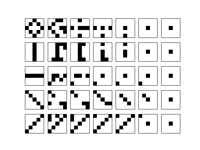
Now the sum is simply the activation of neuron i. As our update rule guarantees that the product of $\Delta s_i$ and the activation of unit i is never negative, this implies that during the upgrade process, the energy function will always increase or stay the same. Thus the state will settle in a local minimum of the energy function.

At this point, we can already see some interesting analogies with the Ising model. Clearly, the units in a Hopfield network correspond to the particles in an Ising model. The state (firing or not) corresponds to the spin (upward or downward). The energy is almost literally the same as the energy of the Ising model without an external magnetic field.

Also the update rules are related. Recall that during a Gibbs sampling step for an Ising model, we calculate the conditional probability

$P = \sigma(2 \beta \langle J_i, s \rangle)$

Here the scalar product is the equivalent of the activation, and we could rewrite this as

$P = \sigma(2 \beta a_i)$

Let us now assume that the temperature is very small, so that $\beta$ is close to infinity. If the activation of unit i is positive, the probability will be very close to one. The Gibbs sampling rule will then almost certainly set the spin to +1. If the activation is negative, the probability will be zero, and we will set the spin to -1. Thus the update role of a Hopfield network corresponds to the Gibbs sampling step for an Ising model at temperature zero.

At nonzero temperatures, a Hopfield network and an Ising model start to behave differently. The Boltzmann distribution guarantees that the state with the lowest energies are most likely, but as the sampling process proceeds, the random element built into the Gibbs sampling rule implies that a state can evolve into another of higher energy as well, even though this is unlikely. For the Hopfield network, the update rule is completely deterministic, and the states will always evolve into states of lower or at least equal energy.

The memories that we are looking for are now the states of minimum energy. If we place the system in a nearby state and let it evolve according to the update rules, it will move over time back into a minimum and thus “remember” the original state.

This is nice, but how do we train a Hopfield network? Given some state s, we want to construct a weight matrix such that s is a local minimum. More generally, if we have already defined weights giving some local minima, we want to adjust the weights in order to create an additional minimum at s, if possible without changing the already existing minima significantly.

In Hopfields paper, this is done with the following learning rule.

$w_{ij} = \begin{cases} \sum_s S^{(s)}_i S^{(s)}_j & i \neq j \\ 0 & i = j \end{cases}$

where $S^{(1)}, \dots, S^{(K)}$ are the states that the network should remember (in a later post in this series, we will see that this rule can be obtained as the low temperature limit of a training algorithm called contrastive divergence that is used to train a certain class of Boltzmann machines).

Thus a state S contributes with a positive value to $w_{ij}$ if $S_i$ and $S_j$ have the same sign, i.e. are in the same state. This corresponds to a rule known as Hebbian learning rule that has been postulated as a principle of learning by D. Hebb and basically states that during learning, connections between neurons are enforced if these neurons fire together ([2], chapter 4).

Let us summarize what we have done so far. We have described a Hopfield network as a fully connected binary neuronal network with symmetric weight matrices and have defined the update rule and the learning rule for these networks. We have seen that the dynamics of the network resembles that of an Ising model at low temperatures. We now expect that a randomly chosen initial state will converge to one of the memorized states and that therefore, this model can serve as an associative memory.

In the next post, we will put this to work and implement and train a Hopfield network in Python to study its actual behavior.

References

1. J. Hopfield, Neural networks and physical systems with emergent collective computational abilities, Proc. Nat. Acad. Sci. Vol. 79, No. 8 (1982), pp. 2554-2558
2. D.O. Hebb, The organization of behaviour, Wiley, New York 1949

On the road again – serializing and deserializing bitcoin transactions

In this post, I will show you how a bitcoin transaction presented in the raw format is to be interpreted and how conversely a bitcoin transaction stored in a C++ (and later Python) object can be converted into a hexadecimal representation (a process called serialization). Ultimately, the goal of this and subsequent posts will be to create a bitcoin transaction from scratch in Python, to sign it and to publish it in a bitcoin network, without using any of the available bitcoin libraries.

The subject of serialization and deserialization in the bitcoin protocol is a bit tricky. At the end of the day, the truth is hidden in the reference implementation somewhere (so time to get the code from the GitHub repository if you have not done so yet). I have to admit that when I first started to work with that code, I found it not exactly easy to understand, given that it has been a few years (well, somewhere around 20 years to be precise) since I last worked with templates in C++. Still, the idea of this post is to get to the bottom of it, and so I will walk you through the most relevant pieces of the source code. But be warned – this will not be an easy read and a bit lengthy. Alternatively, you can also skip directly to the end where the result is again summarized and ignore the details.

The first thing that we need is access to a raw (serialized) bitcoin transaction. This can be obtained from blockchain.info using the following code snippet.

import requests

def get_raw_transaction(txid="ed70b8c66a4b064cfe992a097b3406fa81ff09641fe55a709e4266167ef47891"):
    url = 'https://blockchain.info/en/tx/' + txid + '?format=hex'
    r = requests.get(url)
    return r.text

If you print the result, you should get

0200000003620f7bc1087b0111f76978ef747001e3ae0a12f254cbfb858f
028f891c40e5f6010000006a47304402207f5dfc2f7f7329b7cc731df605
c83aa6f48ec2218495324bb4ab43376f313b840220020c769655e4bfcc54
e55104f6adc723867d9d819266d27e755e098f646f689d0121038c2d1cbe
4d731c69e67d16c52682e01cb70b046ead63e90bf793f52f541dafbdfeff
fffff15fe7d9e0815853738ce47deadee69339e027a1dfcfb6fa887cce3a
72626e7b010000006a47304402203202e6c640c063989623fc782ac1c9dc
3c6fcaed996d852ec876749ba63db63b02207ef86e262ad4b4bc9cebfadb
609f52c35b0105e15d58a5ecbecc5e536d3a8cd8012103dc526ca188418a
b128d998bf80942d66f1b3be585d0c89bd61c533bddbdaa729feffffff84
e6431db86833897bab333d844486c183dd01e69862edea442e480c2d8cb5
49010000006a47304402200320bc83f35ceab4a7ef0f8181eedb5f54e3f6
17626826cc49c8c86efc9be0b302203705889d6aed50f716b81b0f3f5769
d72d1b8a6b59d1b0b73bcf94245c283b8001210263591c21ce8ee0d96a61
7108d7c278e2e715ac6d8afd3fcd158bee472c590068feffffff02ca780a
00000000001976a914811fb695e46e2386501bcd70e5c869fe6c0bb33988
ac10f59600000000001976a9140f2408a811f6d24ab1833924d98d884c44
ecee8888ac6fce0700

Having that, we can now start to go through this byte by byte – you might even want to print that string and strike out the bytes as we go. To understand how serialization works in the reference implementation, we will have to study the the header file serialize.h containing boilerplate code to support serialization. In addition, each individual data type contains specific serialization code. It is useful to compare our results with the human readable description of the transaction at blockchain.info.

To understand how the mechanism works, let us start at the function getrawtransaction in rpc/rawtransaction.cpp which is implementing the corresponding RPC call. This function ends up calling TxToUniv in core_write.cpp and finally EncodeHexTx in the same file. Here an instance of the class CDataStream is created which is defined in streams.h. For that class, the operator << is overwritten so that the function Serialize is invoked. Templates for this method are declared in serialize.h and will tell us how the individual data types are serialized in each individual case for the elementary data types and sets, vectors etc.. All composite classes need to implement their own Serialize method to fit into this scheme.

For a transaction, the method CTransaction::Serialize is defined in primitives/transaction.h and delegates the call to the function SerializeTransaction in the same file.

template
inline void SerializeTransaction(const TxType& tx, Stream& s) {
    const bool fAllowWitness = !(s.GetVersion() & SERIALIZE_TRANSACTION_NO_WITNESS);

    s << tx.nVersion;
    unsigned char flags = 0;
    // Consistency check
    if (fAllowWitness) {
        /* Check whether witnesses need to be serialized. */
        if (tx.HasWitness()) {
            flags |= 1;
        }
    }
    if (flags) {
        /* Use extended format in case witnesses are to be serialized. */
        std::vector vinDummy;
        s << vinDummy;
        s << flags;
    }
    s << tx.vin;
    s << tx.vout;
    if (flags & 1) {
        for (size_t i = 0; i < tx.vin.size(); i++) {
            s << tx.vin[i].scriptWitness.stack;
        }
    }
    s << tx.nLockTime;
}

Throughout this post, we will ignore the extended format that relates to the segregated witness feature and restrict ourselves to the standard format, i.e. to the case that the flag fAllowWitness above is false.

We see that the first four bytes are the version number, which is 2 in this case. Note that little endian encoding is used, i.e. the first byte is the least significant byte. So the version number 2 corresponds to the string

02000000

Next, the transaction inputs and transaction outputs are serialized. These are vectors, and the mechanism for serializing vectors becomes apparent in serialize.h.

template
void Serialize_impl(Stream& os, const std::vector& v, const V&)
{
    WriteCompactSize(os, v.size());
    for (typename std::vector::const_iterator vi = v.begin(); vi != v.end(); ++vi)
        ::Serialize(os, (*vi));
}

template
inline void Serialize(Stream& os, const std::vector& v)
{
    Serialize_impl(os, v, T());
}

We see that to serialize a vector, we first serialize the length of the vector, i.e. the number of elements, and then call the serialization method on each of the individual items. The length is serialized in a compact format called a varInt which stores a number in 1 – 9 bytes, depending on its size. In this case, one byte is sufficient – this is the byte 03 after the version number. Thus we can conclude that the transaction has three transaction inputs.

To understand the next bytes, we need to look at the method CTxIn::SerializeOp.

template
inline void SerializationOp(Stream& s, Operation ser_action) {
    READWRITE(prevout);
    READWRITE(scriptSig);
    READWRITE(nSequence);
}

This is not very surprising – we see that the spent transaction output, the signature script and the sequence number are serialized in that order. The spent transaction prevout is an instance of COutPoint which has its own serialization method. First, the transaction ID of the previous transaction is serialized according to the method base_blob::Serialize defined in uint256.h. This will produce the hexadecimal representation in little endian encoding, so that we have to reverse the order bytewise to obtain the transaction ID.

So in our example, the ID of the previous transaction is encoded in the part starting with 620f7b… in the first line and ending (a transaction ID has always 256 bit, i.e. 32 bytes, i.e. 64 characters) with the bytes …1c40e5f6 early in the second line. To get the real transaction ID, we have to revert this byte for byte, i.e. the transaction ID is

f6e5401c898f028f85fbcb54f2120aaee3017074ef7869f711017b08c17b0f62

The next four bytes still belong to the spent transaction and encode the index of the spent output in the list of outputs of the previous transaction. In this case this is 1, again encoded in little endian byte order, i.e. as 01000000. Thus we have now covered and understood the following part of the hex representation.

0200000003620f7bc1087b0111f76978ef747001e3ae0a12f254cbfb858f
028f891c40e5f601000000

Going back to the serialization method of the class CTxIn, we now see that the next few bytes are the signature script. The format of the signature script is complicated and will be covered in a separate post. For today, we simply take this as a hexadecimal string. In our case, this string starts with 6a473044 …. in the second line and ends with … 541dafbd close to the end of line five.

Finally, the last two bytes in line five and the first two bytes in line six are the sequence number in little endian byte order.

We are now done with the first transaction input. There are two more transaction inputs that follow the same pattern, the last one ends again with the sequence number close to the end of line 15.

Now we move on to the transaction outputs. Again, as this is a vector, the first byte (02) is the number of outputs. Each output is then serialized according to the respective method of the class TxOut.

template
inline void SerializationOp(Stream& s, Operation ser_action) {
    READWRITE(nValue);
    READWRITE(scriptPubKey);
}

The first element is the value, which is an instance of the class CAmount. Again, we can look up the serialization method of this class in amount.h and find that this is simply a 64 bit integer, so its serialization method is covered by the templates in serialize.h and results simply in eight bytes in little endian order:

ca780a0000000000

If we reorder and decode this, we obtain 686282 Satoshi, i.e. 0.0686282 bitcoin. The next object that is serialized is the public key script. Again, we leave the details to a later post, but remark that (which is also true for the signature script) the first byte is the length of the remaining part of the script in bytes, so that we can figure out that the script is composed of the 0x19 = 25 bytes

76a914811fb695e46e2386501bcd70e5c869fe6c0bb33988ac

For the second output, the pattern repeats itself. We have the amount and the public key script

76a9140f2408a811f6d24ab1833924d98d884c44ecee8888ac

of the second output.

Finally, there are four bytes left: 6fce0700. Going back to SerializeTransaction, we identify this as the lock time 0x7ce6f ( 511599 in decimal notation).

After going through all these details, it is time to summarize our findings. A bitcoin transaction is encoded as a hexadecimal string as follows.

The version number (4 bytes, little endian)
The number of transaction inputs
For each transaction input:
- the ID of the previous transaction (reversed)
- the index of the spent transaction output in the previous transaction (4 bytes, little endian)
- the length of the signature script
- the signature script
- the sequence number (4 bytes, little endian)
The number of transaction outputs
For each transaction output:
- the amount (eight bytes, little endian encoding) in Satoshi
- the length of the public key script
- the public key script
the locktime (four bytes, little endian)

In my GitHub account, you will find a Python script Transaction.py that retrieves our sample transaction from the blockchain.info site and prints out all the information line by line. To run it, clone the repository using

$ git clone https://github.com/christianb93/bitcoin.git ; cd bitcoin

and then run the script

$ python Transaction.py

The script uses a few modules in the package btc, namely txn.py and serialize.py that essentially implement the serialization and deserialization routines discussed in this post.

That is it for today. In the next posts, I will start to look at a topic that we have more or less consequently ignored or oversimplified so far: scripts in the bitcoin world.

Transactions in the bitcoin network

In my previous posts on the bitcoin protocol, I have described those objects that constitute participants – private and public keys and bitcoin addresses. Now we will look at those objects that represent actual transfers of bitcoins between these participants, namely at transactions.

Essentially, a bitcoin transaction consists of two parts. First, a transaction contains a list of one or more transaction outputs. A transaction output describes the target of the bitcoin transfer and basically consists of a recipient, usually identified by the bitcoin address, and an amount that this recipient is supposed to receive. A transaction can have one or more outputs and thus pay bitcoins to different recipients as part of one transaction (in fact, this is typically the case due to the need for change as we will see later).

There are different types of transaction outputs. The most common one is called a Pay to Public Key Hash (P2PKH) transaction output and refers to a recipient by a hash of the public key of that recipient, which is essentially the same as the bitcoin address. Only the owner of that public key, i.e. technically speaking whoever has access to the private key, can spend these transaction outputs – we will see later how the signing process in the blockchain takes care of this.

Similar to outputs, that determine the target of the payment, there are transaction inputs, that determine the source of the payment. Each transaction input refers to an earlier transaction output. Transaction outputs that are also consumed by some transaction input are called spent, outputs that are not yet referenced by any transaction input are called unspent transaction outputs, abbreviated UTXO.

Let us look at an example to illustrate this. Suppose Alice wants to transfer 1.0 BTC to Bob. She (respectively her wallet software) will first scan all the unspent transaction outputs available to Alice, i.e. all transaction outputs that refer to public keys for which Alice has the private key. In the example displayed above, her wallet might locate two transactions (the transactions on the left of the picture) that together contain three transaction outputs with amounts 0.3, 0.5 and 0.4 (the outputs not circled in red).

These outputs sum up to 1.2 BTC and are therefore sufficient to fund the payment to Bob. Alice will therefore construct a transaction – displayed in the middle of the picture above – that has three inputs, each of them referring to the selected transaction outputs. She could now try to add only one output to the transaction and put Bobs public key hash into this output, but this would mean that she transfers 1.2 BTC to Bob, not only 1.0 BTC. Therefore Alice will add a second transaction output to her transaction, that transfers a certain amount called the change back to herself. Many wallets use dedicated addresses for this that are called change addresses.

In the example above, the change – represented by the second transaction output – is 0.1 BTC. Thus the total inputs of the transaction sum up to 1.2 BTC, the total outputs sum up to 1.1 BTC. The difference is called the fee and will be credited to the miner who creates the block in which the transaction will be included – we will look at the process in mining in a separate post.

We now see that there is no such thing as a “bitcoin balance” stored somewhere in the blockchain. There are only transactions, and ownerhip of bitcoin is equivalent to owning the private key that matches unspent transaction outputs. Transactions form a chain, where each transaction is linked to previous transactions via the transaction inputs, and this chain represents the flow of bitcoin ownership.

You might ask yourself whether this is not a “chicken and egg” problem. If each transaction can only spend bitcoins that are present in previously unspent transaction outputs, where do all the bitcoins initially come from? The answer is again provided by the process of mining, where special bitcoin transactions called coinbase transactions are generated that only have an output (and a dummy input) so that bitcoin supply is created.

With this preparation, let us now take a look at the source code of the reference implementation. The transaction data structure is defined in primitives/transaction.h. After removing some comments and constants, the relevant part of the code is

class CTransaction
{
public:
    const int32_t nVersion;
    const std::vector vin;
    const std::vector vout;
    const uint32_t nLockTime;

We see that in addition to the attributes that we expect – a vector of transaction inputs and a vector of transaction outputs – a transaction has two additional attributes. The first attribute is the version number. The current version number is 2 (CURRENT_VERSION in the header file), but you will also find older transactions with version number one. The second additional field is the locktime, which can be used to define an earliest time (or block) at which the transaction can be added to the chain.

In the same header file, the transaction input and the transaction output structure are defined. We start with the transaction output.

class CTxOut
{
public:
CAmount nValue;
CScript scriptPubKey;

We see that a transaction output consists of a value that represents the amount that the transaction transfers, and a field called scriptPubKey which contains essentially the hash of the public key of the recipient – we will look at scripts in the bitcoin protocol in more detail in a later post. The definition of CAmount is located in amount.h:

/** Amount in satoshis (Can be negative) */
typedef int64_t CAmount;

static const CAmount COIN = 100000000;
static const CAmount CENT = 1000000;

The amount is thus specified in a unit called Satoshi which is therefore the smallest unit of bitcoin that can be transferred. The constant COIN is the number of Satoshi that comprises one bitcoin and is $10^8$ .

The definition of the transaction input is similar. Ignoring a feature called segregated witness, the relevant part is

class CTxIn
{
public:
COutPoint prevout;
CScript scriptSig;
uint32_t nSequence;

Here COutPoint is a class that refers to a previous transaction output – the spent transaction output – as expected from the picture above, and which consists of the ID (i.e. hash value) of the transaction that contains the previous output as well as the index of the output in the vector of all transaction outputs of this transaction. The attribute scriptSig contains roughly speaking a signature of the entire transaction that has been produced with the private key that belongs to the public key referenced in the spent transaction output. Finally, the field nSequence is called the sequence number and can be used in combination with the locktime – again we will not get into details on this in this post yet.

The image above summarizes what we have learned so far about the structure of a bitcoin transaction. Time to take a look at a real transaction. The page blockchain.info offers an API to retrieve transactions from the bitcoin blockchain. So let us open a terminal and enter

$ curl https://blockchain.info/en/tx/ed70b8c66a4b064cfe992a097b3406fa81ff09641fe55a709e4266167ef47891?format=hex 0200000003620f7bc1087b0111f76978ef747001e3ae0a12f254cbfb858f028f891c40e5f6010000006a47304402207f5dfc2f7f7329b7cc731df605c83aa6f48ec2218495324bb4ab43376f313b840220020c769655e4bfcc54e55104f6adc723867d9d819266d27e755e098f646f689d0121038c2d1cbe4d731c69e67d16c52682e01cb70b046ead63e90bf793f52f541dafbdfefffffff15fe7d9e0815853738ce47deadee69339e027a1dfcfb6fa887cce3a72626e7b010000006a47304402203202e6c640c063989623fc782ac1c9dc3c6fcaed996d852ec876749ba63db63b02207ef86e262ad4b4bc9cebfadb609f52c35b0105e15d58a5ecbecc5e536d3a8cd8012103dc526ca188418ab128d998bf80942d66f1b3be585d0c89bd61c533bddbdaa729feffffff84e6431db86833897bab333d844486c183dd01e69862edea442e480c2d8cb549010000006a47304402200320bc83f35ceab4a7ef0f8181eedb5f54e3f617626826cc49c8c86efc9be0b302203705889d6aed50f716b81b0f3f5769d72d1b8a6b59d1b0b73bcf94245c283b8001210263591c21ce8ee0d96a617108d7c278e2e715ac6d8afd3fcd158bee472c590068feffffff02ca780a00000000001976a914811fb695e46e2386501bcd70e5c869fe6c0bb33988ac10f59600000000001976a9140f2408a811f6d24ab1833924d98d884c44ecee8888ac6fce0700

The curl command (you could also open the URL in a browser) retrieves a transaction in raw hexadecimal format, specifying the transaction ID as an input (the transaction ID is essentially a hash of the transaction, more on this later). The output is a hexadecimal string containing the requested transaction. This is called a serialized version of the transaction and is important for a number of reasons. First, this is the format that goes over the wire if two nodes in the bitcoin network exchange the transaction. Second, when a transaction is signed, included in a block or when its transaction ID is formed, this serialized representation is the basis. In the next post in this series, we will learn how to encode this representation to match it with the structure described above.

Until then, you might want to play around with the transaction browser at bitcoin.info – just remove the ?format=hex from the URL above and you will get a human readable version of the transaction which will allow you to locate some of the elements (inputs, outputs and amounts) discussed in this post.

Keys in the bitcoin network: the public key

In my last post, we have looked in some detail at the private key – how it is generated and how it can be decoded and stored. Let us now do the same with the public key.

Recall that a public key is simply a point on the elliptic curve SECP256K1 that is used by the underlying ECDSA algorithm – in fact it is obtained by multiplying the generator point on the curve by our private key. As any point on the curve, it therefore has an x-coordinate and a y-coordinate, both being 32 bytes unsigned integers. So one way to encode the public key would be as follows.

take the x-coordinate as a point, represented by an integer smaller than p
convert this into a 32 byte hexadecimal string, using for instance big endian encoding
do the same for the y-coordinate
and concatenate these two strings to obtain a single 64 byte hexadecimal string

This encoding is simple, but it has a drawback. Remember that we encode not just a random pair of integers, but a point on the curve, so the x-coordinate and y-coordinate are related by the curve equation

$y^2 = x^3 + ax + b$

Thus given x, we almost know y – we know the square of y modulo p, and there can be at most two different roots of this equation. So we could reconstruct y if we have x and an additional bit that tells us which of the two solutions we need.

Let us now assume that p is odd. If y is a solution of the equation for a given value of x, then p – y (which is -y modulo p) is the second solution. As p is odd, exactly one of the two numbers y and p – y is even. We can therefore use an additional bit that is equal to y modulo 2 to distinguish the two solutions. It is convention to store this bit in a full additional byte, using the value 2 if y is even and the value 3 if y is odd, so that we obtain a representation of the public key (and in fact any other point on the curve) in at most 33 bytes: at most 32 bytes for the value of the x-coordinate and the additional byte containing the value of y modulo 2. This representation is called the compressed representation (see for instance the publication of the SECG, section 2.3).

If there is a compressed representation, you might expect that there is also an uncompressed representation. This is simply the representation that we have described above, i.e. storing both x and y, with an additional twist: to be able to distinguish this from a compressed representation that always starts with 0x02 or 0x03, a leading byte with value 0x04 is added so that the total length of an uncompressed representation is at most 65 bytes. Since version 0.6.0, the bitcoin reference implementation defaults to using compressed keys (see the function CWallet::GenerateNewKey).

Let us summarize what we have learned so far in a short Python code snippet that will take a private key (stored as integer in the variable d), calculate the corresponding point on the elliptic curve SECP256K1 using the ECDSA library and create a compressed representation of the result.

#
# Determine the public key from the
# secret d
#
import ecdsa
curve = ecdsa.curves.SECP256k1
Q = d * curve.generator
#
# and assemble the compressed representation
#
x = Q.x()
y = Q.y()
pubKey = x.to_bytes(length=32, byteorder="big")
pubKey = binascii.hexlify(pubKey).decode('ascii')
if 1 == (y % 2):
    pubKey = "03" + pubKey
else:
    pubKey = "02" + pubKey
print("Compressed key:  ", pubKey)

This way of encoding a public key is in fact not specific to the bitcoin network, but a standard that is used whenever a point on an elliptic curve needs to be encoded – see for instance RFC5480 by the IETF which is part of the X.509 standard for certificates.

However, this is still a bit confusing. If you known the nuts and bolts of the bitcoin protocol a bit, you will have seen that participants publish something that is called an address which is a string similar to

mx5zVKcjohqsu4G8KJ83esVxN52XiMvGTY

That does not look at all like a compressed or uncompressed public key. We are missing something.

The answer is that an address is in fact not a public key, but it is derived from a public key. More precisely, it is an encoded version of a hash value of the public key. So given the address, it is easy to verify that this address belongs to a certain public key, but it is very hard to reconstruct the public key given the address.

To understand the relation between a public key and an address better, it is again time to take a look at the source code of the reference client. A good starting point is the RPC method getnewaddress. This method is defined in the file wallet/rpcwallet.cpp and creates an instance of the class CBitcoinAddress which in turn is – surprise – derived from our old friend CBase58Data. The comments are quite helpful, and it is not difficult to figure out that a bitcoin address is obtained as follows from a public key.

create a hexadecimal compressed representation of the public key
apply a double hash to turn this into a sequence of 20 bytes – first apply the hash algorithm SHA256, then RIPEMD160 (this is called a Hash160 in the bitcoin terminology as the output will have 160 bits)
add a prefix to mark this as a public key address – the prefix is again defined in chainparams.cpp and and is zero for the main network and 111 for the test networks
take the hash256 checksum and append the first four bytes
apply Base58 decoding to the result

This is already very similar to what we have seen before and can be done in a few lines of Python code.

def hash160(s):
    _sha256 = hashlib.sha256(s).digest()
    return hashlib.new("ripemd160", _sha256).digest()
#
# Apply hash160
#
keyId = hash160(bytes.fromhex(pubKey))
#
# Append prefix for regtest network
#
address = bytes([111]) + keyId
#
# Add checksum
#
chk = hash256(address)[:4]
#
# and encode
#
address = btc.utils.base58Encode(address + chk)
print("Address:         ", address)

Heureka! If we run this, we get exactly the address mx5zVKcjohqsu4G8KJ83esVxN52XiMvGTY that the bitcoin client returned when we started our little journey at the beginning of the post on private keys.

As always, the full source code is also available on GitHub repository. If you want to run the code, simply enter

$ git clone https://github.com/christianb93/bitcoin.git
$ cd bitcoin
$ python Keys.py

That was it for today. We have now covered the basics of what constitutes participants in the bitcoin network. In the next few posts in this series. we will look at the second main object in the bitcoin world – transactions. We will learn how to interpret transactions, and will eventually be able to manually create a transaction to instruct a payment, sign it, hand it over to our test network and see how it is processed.

Keys in the bitcoin network: the private key

In my last post, I have shown you how arithmetic on elliptic curves can be used to create and verify digital signatures. We have seen that every party that creates a signature is represented by a private key – kept securely – and a public key, which is made available to everyone who wants to verify the signature. In a blockchain, digital signatures are used to verify ownership of bitcoins, and therefore private and public keys play a pivotal role in the bitcoin network. Bitcoin transaction outputs refer to public keys, and only the person that is in control of the matching private key can spend the bitcoin. Thus it is worth to take a closer look at how keys are represented in the bitcoin protocol.

Bitcoin uses the ECDSA signature algorithm to sign messages and verify signatures. Therefore a private key in the bitcoin network is simply an integer. More precisely, it is an integer between one and the order of the generator of an elliptic curve SECP256K1 (if that sounds like gibberish to you, you should read my previous post on this). Generating private keys is therefore very easy – you simply randomly select a 32 byte integer until you find one which is below that order (I am cheating a bit – obviously you need a good source of random numbers for this which makes it hard to predict the private key). I have done that for you:

$d = 103028256105408389446438916672504271192164767440296751065327418112299269382535$

Of course that is not a private key that I really use – it would not be smart to publish it if it were. But it is a perfectly valid private key. Unfortunately, this is not the way how a private key is typically stored and presented by a bitcoin client. In fact, what I did to create this key is to run the commands


$ bitcoin-cli -regtest getnewaddress "myAccount"

mx5zVKcjohqsu4G8KJ83esVxN52XiMvGTY

$ bitcoin-cli -regtest dumpprivkey "mx5zVKcjohqsu4G8KJ83esVxN52XiMvGTY"

cVDUgUEahS1swavidSk1zdSHQpCy1Ac9XSQHkaxmZKcTTfEA5vTY

after installing the reference bitcoin core software on my computer. The last line is the private key – and that looks very much different from the number d above (you do not necessarily need a bitcoin installation to follow this post, but you will definitely need it to run all the examples in future posts, so this might be a good point in time to stop and install it. So go to the download page, get the version for your machine and install it. Do not forget to start the bitcoin daemon in regtest mode, if you want to avoid downloading the full blockchain with more than 200 GBytes at the time of writing. In my bitcoin configuration file bitcoin.conf located in the directory ~/.bitcoin, I have set the options

regtest=1
server=1

to tell bitcoin to accept RPC commands and to run in regression test mode. But back to keys now …).

The funny string that the bitcoin client will present you as the private key is in fact an encoded private key using the WIF format (wallet interchange format). Let us try to understand how we can convert this into the number d displayed above.

The first thing you need to know about a WIF encoded private key is that it is encoded using the Base58 standard. Similar to Base64 (which an official IETF standard described in RFC4648), this is a standard to encode a number in a way that can easily be transmitted over channels like e-mail or even printed on paper without having to deal with binary values. Essentially, the idea is that we use an alphabet of 58 ASCII characters and to convert the number to the base 58, representing each digit by the corresponding character from this alphabet. In addition, there is some logic to handle leading zeros, more precisely to avoid that they are dropped during the conversion. If you want to see all this in detail, the authorative answer is (as always) the source code of the module base58c.cpp in the C++ reference implementation which is hosted on GitHub.

To do this in Python, we have – as always – several choices. We can search for a library that performs Base58 encoding and decoding – for instance https://github.com/keis/base58. For the sake of demonstration, I have created my own routines. To decode, i.e. to turn a Base58 string into a sequence of bytes, the following code will do.


BASE58_ALPHABET = '123456789ABCDEFGHJKLMNPQRSTUVWXYZabcdefghijkmnopqrstuvwxyz'
def base58_decode(s):
    #
    # Strip off leading 1's as these represent leading
    # zeros in the original
    #
    zeros = 0
    while (zeros < len(s)) and (s[zeros] == '1'):
        zeros = zeros + 1
    s = s[zeros:]
    #
    # We first turn the string into an integer
    #
    value, power = 0, 1
    for _ in reversed(s):
        value += power * BASE58_ALPHABET.index(_)
        power = power * 58
    #
    # Now convert this integer into a sequence of bytes
    #
    result = value.to_bytes((value.bit_length() + 7) // 8, byteorder='big')
    #
    # and append the leading zeros again
    #
    for _ in range(zeros):
        result = (0).to_bytes(1, 'big') + result
    return result

I have stored this in a module btc.utils for later use, which you can find, along with the other examples from this post, in my GitHub repository.

Let us now apply this to our example WIF file.

import binascii
import btc.utils

#
# The WIF encoded private key
#
wif = "cVDUgUEahS1swavidSk1zdSHQpCy1Ac9XSQHkaxmZKcTTfEA5vTY"
print("WIF:    ", wif)
#
# Convert into a sequence of bytes
#
b = btc.utils.base58_decode(wif)
#
# and into hex
#
h = binascii.hexlify(b).decode('ascii')
print("Hex:    ", h)

If you run this code, you will find that the output has 76 characters, i.e. 76 / 2 = 38 bytes. That cannot be quite right, because we expect that our private key is an integer with 32 bytes only. So there are six extra bytes. Where do they come from?

To get used to it, let us again try to find the answer in the source code of the reference implementation (you can browse the code in the GitHub repository online or (recommended) clone to obtain a local copy so that you can use tools like grep and their friends. As a starting point, remember that we have received our private key via the bitcoin-cli tool that communicates with the bitcoin server via RPC calls, and that we have used the RPC method dumpprivatekey. So let us search for that.


(cd bitcoin/src ; grep -R -I "dumpprivkey" *)

That will give you a few matches in two files,wallet/rcpwallet.cpp and wallet/rpcdump.cpp. If you open these two files and look at the code, you will find that the former refers to the latter. This function first retrieves the key from the wallet and then creates an instance of the class CBitcoinSecret (which is derived from CBase58Data and invokes its ToString() method to obtain the textual representation of the key that is then returned.

One more usage of grep will tell you that the code for these classes is located in the file base58.cpp which we have already met. The constructor calls CBitcoinSecret::SetKey() and the method ToString() is implemented in the base class, so we also need to look at CBase58Data::ToString(). Going carefully through this code, we find that the data is actually composed of four parts.

The first byte is a version number which is used to distinguish a private key used for the testnet (239) from a key for the productive network (128) (look up the values in chainparams.cpp). The next few bytes are the actual secret d, encoded as a hexadecimal string using big endian encoding (i.e. the most significant octet first). The next byte is a flag that describes whether the public key that belongs to this private key should be stored in compressed format or not. We will get back to this point in a later post on public keys and addresses, for the time being we can safely ignore this byte.

The last four bytes are again interesting. They form a checksum for the remainder. These four bytes are obtained by applying what is called a Hash256 in the bitcoin language and which is just a double SHA256 hash, and then taking the first four bytes of the result. Thus in order to turn the WIF string into a number, we have to decode it using Base58, strip off the last four bytes, verify the checksum, strip off one additional byte, remove the trailing version number and convert the remaining hexadecimal string into an integer.

import binascii
import btc.utils
import hashlib

def hash256(s):
    return hashlib.sha256(hashlib.sha256(s).digest()).digest()

#
# The WIF encoded private key
#
wif = "cVDUgUEahS1swavidSk1zdSHQpCy1Ac9XSQHkaxmZKcTTfEA5vTY"
print("WIF:       ", wif)
#
# Convert into a sequence of bytes
#
b = btc.utils.base58_decode(wif)
#
# and into hex
#
h = binascii.hexlify(b).decode('ascii')
print("Hex:       ", h)
#
# Strip off checksum
#
chk = h[-8:]
print("Checksum:  ", chk)
h = h[:-8]
#
# and verify it
#
_chk = hash256(bytes.fromhex(h))[:4]
assert(_chk == bytes.fromhex(chk))
#
# Strip off version byte
#
print("Version:   ", int(h[:2], 16))
h = h[2:]
#
# and compression flag
#
h = h[:-2]

d = int.from_bytes(bytes.fromhex(h), "big")
print("Secret:    ", d)

If you run this, you should get the value for d that we started with at the beginning of this post.

We have now seen how private keys can be generated and encoded. Typically private keys are kept in a wallet, but they could also be printed out in their WIF encoded form and stored offline – you could even create a private key on a machine not connected to any network and store it in this way. This is called a paper wallet in the bitcoin world.

But what about the public key? If you want to receive bitcoins, the payee needs access to your public key or at leat to a condensed version of it called the bitcoin address. We have seen that for the ECDSA algorithm, the public key can be calculated given the private key, and we will see that the address can in turn be calculated given the public key. In my next post, I will guide you through this process.