christianb93

Virtual networking labs – building a virtual router with iptables and Linux namespaces

When you are trying to understand virtual networking, container networks, micro segmentation and all this, sooner or later the day will come where you will have to deal with iptables, the built-in Linux firewall mechanism. After evading the confrontation with the full complexity of this remarkable beast for many years, I have recently decided to dive a little deeper into the internals of the Linux networking stack. Today, I will give you an overview of the inner workings of the machinery behind iptables and show you how to use this to build a virtual firewall in a Linux networking namespace.

Netfilter hooks in the Linux kernel

In order to understand how iptables work, we will have to take a short look at a mechanism called netfilter hooks in the Linux networking stack.

Netfilter hooks are points in the Linux networking code at which modules can add their own custom processing. When a packet is travelling up or down through the networking stack and reaches one of these points, it is handed over to the registered modules which can manipulate the packet and, by their return value, can either instruct the core networking code to continue with the processing of the packet or to drop it.

Let us take a closer look at where these netfilter hooks are placed in the kernel. The following diagram is a (simplified) summary of the way that packets take through the Linux IPv4 stack (for those readers who actually want to see this in the Linux kernel code, I have added some of the most relevant Linux kernel functions, referring to v4.2 of the kernel).

A packet coming in from a network device will first reach the pre-routing hook. As the name indicates, this happens before a routing decision is taken. After passing this hook, the kernel will consult its routing tables. If the target IP address is the IP address of a local device, it will flag the packet for local delivery. These packets will now be processed by the input hook before they are handed over to the higher layers, e.g. a socket listening on a port.

If the routing algorithm determines that the packet is not targeted towards a local interface but needs to be forwarded, the path through the kernel is different. These packets will be handled by the forwarding code and pass the forward netfilter hook, followed by the post-routing hook. Then, the packet is sent to the outgoing network interface and leaves the kernel.

Finally, for packets that are locally generated by an application, the kernel first determines the route to the destination. Then, the modules registered for the output hook are invoked, before we also reach the post-routing hook as in the case of forwarding.

Having discussed netfilter hooks in general, let us now turn to iptables. Essentially, iptables is a framework sitting on top of the netfilter hooks which allows you to define rules that are evaluated at each of the hooks and determine the fate of the packet. For each netfilter hook, a set of rules called a chain is processed. Consequently, there is an input chain, an output chain, a pre-routing chain, a post-routing chain and a forward chain. If it also possible to define custom chains to which you can jump from one of the pre-built chains.

Iptables rules are further organized into tables and wired up with the kernel code using netfilter hooks, but not every table registers for every hook, i.e. not every table is represented in every chain. The following diagram shows which chain is present in which table.

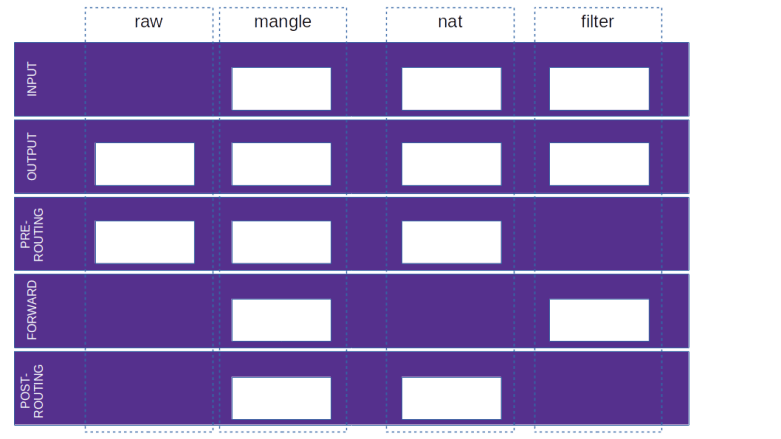
It is sometimes stated that iptables chains are contained in tables, but given the discussion of netfilter hooks above, I prefer to think of this a matrix – there are chains and tables, and rules are sitting at the intersections of chains and tables, so that every rule belongs to a table and a chain. To illustrate this, let us look at the processing steps taken by iptables for a packet for a local destination.

Process the rules in the raw table in the pre-routing chain
Process the rules in the mangle table in the pre-routing chain
Process the rules in the nat table in the pre-routing chain
Process the rules in the mangle table in the input chain
Process the rules in the nat table in the input chain
Process the rules in the filter table in the input chain

Thus, rules are evaluated at every point in the above diagram where a white box indicates a non-empty intersection of tables and chains.

Iptables rules

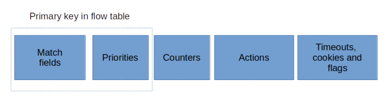
Let us now see how the actual iptables rules are defined. Each rule consists of a match which determines to which packets the rule applies, and a target which determines the action taken on the packet. Some targets are terminating, meaning that the processing of the packet stops at this point, other targets are non-terminating, meaning that a certain action will be taken and processing continues. Here are a few examples of available targets, see the documentation listed in the last section for the full specification.

Action	Description
ACCEPT	Accept the packet, i.e do not apply any further rules within this combination of chain and table and instruct the kernel to let the packet pass
DROP	Drop the packet, i.e. tell the kernel to stop processing of the packet without any further action
REJECT	Tell the kernel to stop processing of the packet and send an ICMP reject message back to the origin of the packet
SNAT	Perform source NATing on the packet, i.e. change the source IP address of the packet, more on this below
DNAT	Destination NATing, i.e. change the destination IP address of the packet, again we will discuss this in a bit more detail below
LOG	Log the packet and continue processing
MARK	Mark the packet, i.e. attach a number which can again be used for matching in a subsequent rule

Note, however, that not every action can be used in every chain, but certain actions are restricted to specific tables or chains

Of course, it might happen that no rule matches. In this case, the default target is chosen, which is also known as the policy for a given table and chain.

As already mentioned above, it is also possible to define custom chains. These chains can be used as a target, which implies that processing will continue with the rules in this chain. From this chain, one can either return explicitly to the original table using the RETURN target, or, otherwise, the processing continues in the original table once all rules in the custom chain have been processed, so this is very similar to a function or subroutine in a high-level language.

Setting up our test lab

After all this theory, let us now see iptables in action and add some simple rules. First, we need to set up our lab. We will simulate a situation where two hosts, called boxA and boxB are connected via a router, as indicated in the following diagram.

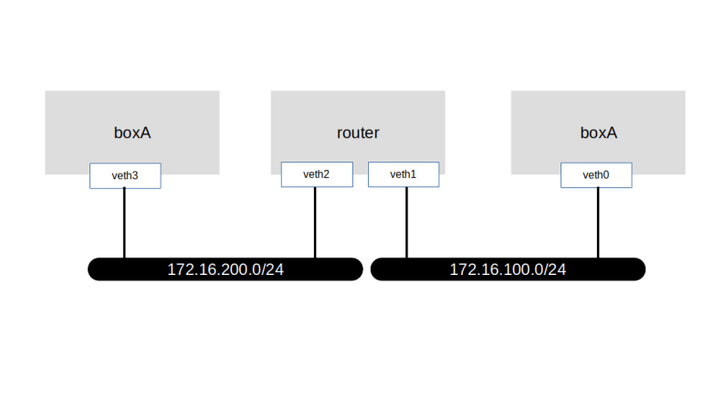
We could of course do this using virtual machines, but as a lightweight alternative, we can also use IP namespaces (it is worth mentioning that similar to routing tables, iptables rules are per namespace). Here is a script that will set up this lab on your local machine.

	# Create all namespaces
	sudo ip netns add boxA
	sudo ip netns add router
	sudo ip netns add boxB

	# Create veth pairs and move them into their respective namespaces
	sudo ip link add veth0 type veth peer name veth1
	sudo ip link set veth0 netns boxA
	sudo ip link set veth1 netns router
	sudo ip link add veth2 type veth peer name veth3
	sudo ip link set veth3 netns boxB
	sudo ip link set veth2 netns router

	# Assign IP addresses
	sudo ip netns exec boxA ip addr add 172.16.100.5/24 dev veth0
	sudo ip netns exec router ip addr add 172.16.100.1/24 dev veth1
	sudo ip netns exec boxB ip addr add 172.16.200.5/24 dev veth3
	sudo ip netns exec router ip addr add 172.16.200.1/24 dev veth2

	# Bring up devices
	sudo ip netns exec boxA ip link set dev veth0 up
	sudo ip netns exec router ip link set dev veth1 up
	sudo ip netns exec router ip link set dev veth2 up
	sudo ip netns exec boxB ip link set dev veth3 up

	# Enable forwarding globally
	echo 1 > /proc/sys/net/ipv4/ip_forward

	# Enable logging from within a namespace
	echo 1 > /proc/sys/net/netfilter/nf_log_all_netns

view raw

setupLab13.sh

hosted with ❤ by GitHub

Let us now start playing with this setup a bit. First, let us see what default policies our setup defines. To do this, we need to run the iptables command within one of the namespaces representing the different virtual hosts. Fortunately, ip netns exec offers a very convenient way to do this – you simply pass a network namespace and an arbitrary command, and this command will be executed within the respective namespace. To list the current content of the mangle table in namespace boxA, for instance, you would run

sudo ip netns exec boxA \
   iptables -t mangle -L

Here, the switch -t selects the table we want to inspect, and -L is the command to list all rules in this table. The output will probably depend on the Linux distribution that you use. Hopefully, the tables are empty, and the default target (i.e. the policy) for all chains is ACCEPT (no worries if this is not the case, we will fix this further below). Also note that the output of this command will not contain every possible combination of tables and chains, but only those which actually are allowed by the diagram above.

To be able to monitor the incoming and outgoing traffic, we now create our first iptables rule. This rule uses a special target LOG which simply logs the packet so that we can trace the flow through the involved hosts. To add such a rule to the filter table in the OUTPUT chain of boxA, enter

sudo ip netns exec boxA \
   iptables -t filter -A OUTPUT \
   -j LOG \
   --log-prefix "boxA:OUTPUT:filter:" \
   --log-level info

Let us briefly through this command to see how it works. First, we use the ip netns exec command to run a command (iptables in our case) inside a network namespace. Within the iptables command, we use the switch -A to add a new rule in the output chain, and the switch -t to indicate that this rule belongs to the filter table (which, actually, is the default if -t is omitted).

The switch -j indicates the target (“jump”). Here, we specify the LOG target. The remaining switches are specific parameters for the LOG target – we define a log prefix which will be added to every log message and the log level with which the messages will appear in the kernel log and the output of dmesg.

Again, I have created a script that you can run (using sudo) to add logging rules to all relevant combinations of chains and tables. In addition, this script will also add logging rules to detect established connections, more on this below, and will make sure that all default policies are ACCEPT and that no other rules are present.

Let us now run try our first ping. We will try to reach boxB from boxA.

sudo ip netns exec boxA \
   ping -c 1 172.16.200.5

This will fail with the error message “Network unreachable”, as expected – we do have a route to the network 172.16.100.0/24 on boxA (which the Linux kernel creates automatically when we bring up the interface) but not for the network 172.16.200.0/24 that we try to reach. To fix this, let us now add a route pointing to our router.

sudo ip netns exec boxA \
   ip route add default via 172.16.100.1

When we now try a ping, we do not get an error message any more, but the ping still does not succeed. Let us use our logs to see why. When you run dmesg, you should see an output similar to the sample output below.

[ 5216.449403] boxA:OUTPUT:raw:IN= OUT=veth0 SRC=172.16.100.5 DST=172.16.200.5 LEN=84 TOS=0x00 PREC=0x00 TTL=64 ID=15263 DF PROTO=ICMP TYPE=8 CODE=0 ID=20237 SEQ=1 
[ 5216.449409] boxA:OUTPUT:mangle:IN= OUT=veth0 SRC=172.16.100.5 DST=172.16.200.5 LEN=84 TOS=0x00 PREC=0x00 TTL=64 ID=15263 DF PROTO=ICMP TYPE=8 CODE=0 ID=20237 SEQ=1 
[ 5216.449412] boxA:OUTPUT:nat:IN= OUT=veth0 SRC=172.16.100.5 DST=172.16.200.5 LEN=84 TOS=0x00 PREC=0x00 TTL=64 ID=15263 DF PROTO=ICMP TYPE=8 CODE=0 ID=20237 SEQ=1 
[ 5216.449415] boxA:OUTPUT:filter:IN= OUT=veth0 SRC=172.16.100.5 DST=172.16.200.5 LEN=84 TOS=0x00 PREC=0x00 TTL=64 ID=15263 DF PROTO=ICMP TYPE=8 CODE=0 ID=20237 SEQ=1 
[ 5216.449416] boxA:POSTROUTING:mangle:IN= OUT=veth0 SRC=172.16.100.5 DST=172.16.200.5 LEN=84 TOS=0x00 PREC=0x00 TTL=64 ID=15263 DF PROTO=ICMP TYPE=8 CODE=0 ID=20237 SEQ=1 
[ 5216.449418] boxA:POSTROUTING:nat:IN= OUT=veth0 SRC=172.16.100.5 DST=172.16.200.5 LEN=84 TOS=0x00 PREC=0x00 TTL=64 ID=15263 DF PROTO=ICMP TYPE=8 CODE=0 ID=20237 SEQ=1 
[ 5216.449437] router:PREROUTING:raw:IN=veth1 OUT= MAC=c6:76:ef:89:cb:ec:96:ad:71:e1:0a:28:08:00 SRC=172.16.100.5 DST=172.16.200.5 LEN=84 TOS=0x00 PREC=0x00 TTL=64 ID=15263 DF PROTO=ICMP TYPE=8 CODE=0 ID=20237 SEQ=1 
[ 5216.449441] router:PREROUTING:mangle:IN=veth1 OUT= MAC=c6:76:ef:89:cb:ec:96:ad:71:e1:0a:28:08:00 SRC=172.16.100.5 DST=172.16.200.5 LEN=84 TOS=0x00 PREC=0x00 TTL=64 ID=15263 DF PROTO=ICMP TYPE=8 CODE=0 ID=20237 SEQ=1 
[ 5216.449443] router:PREROUTING:nat:IN=veth1 OUT= MAC=c6:76:ef:89:cb:ec:96:ad:71:e1:0a:28:08:00 SRC=172.16.100.5 DST=172.16.200.5 LEN=84 TOS=0x00 PREC=0x00 TTL=64 ID=15263 DF PROTO=ICMP TYPE=8 CODE=0 ID=20237 SEQ=1 
[ 5216.449447] router:FORWARD:mangle:IN=veth1 OUT=veth2 MAC=c6:76:ef:89:cb:ec:96:ad:71:e1:0a:28:08:00 SRC=172.16.100.5 DST=172.16.200.5 LEN=84 TOS=0x00 PREC=0x00 TTL=63 ID=15263 DF PROTO=ICMP TYPE=8 CODE=0 ID=20237 SEQ=1 
[ 5216.449449] router:FORWARD:filter:IN=veth1 OUT=veth2 MAC=c6:76:ef:89:cb:ec:96:ad:71:e1:0a:28:08:00 SRC=172.16.100.5 DST=172.16.200.5 LEN=84 TOS=0x00 PREC=0x00 TTL=63 ID=15263 DF PROTO=ICMP TYPE=8 CODE=0 ID=20237 SEQ=1 
[ 5216.449451] router:POSTROUTING:mangle:IN= OUT=veth2 SRC=172.16.100.5 DST=172.16.200.5 LEN=84 TOS=0x00 PREC=0x00 TTL=63 ID=15263 DF PROTO=ICMP TYPE=8 CODE=0 ID=20237 SEQ=1 
[ 5216.449452] router:POSTROUTING:nat:IN= OUT=veth2 SRC=172.16.100.5 DST=172.16.200.5 LEN=84 TOS=0x00 PREC=0x00 TTL=63 ID=15263 DF PROTO=ICMP TYPE=8 CODE=0 ID=20237 SEQ=1 
[ 5216.449474] boxB:PREROUTING:raw:IN=veth3 OUT= MAC=2a:12:10:db:37:49:a6:cd:a5:c0:7d:56:08:00 SRC=172.16.100.5 DST=172.16.200.5 LEN=84 TOS=0x00 PREC=0x00 TTL=63 ID=15263 DF PROTO=ICMP TYPE=8 CODE=0 ID=20237 SEQ=1 
[ 5216.449477] boxB:PREROUTING:mangle:IN=veth3 OUT= MAC=2a:12:10:db:37:49:a6:cd:a5:c0:7d:56:08:00 SRC=172.16.100.5 DST=172.16.200.5 LEN=84 TOS=0x00 PREC=0x00 TTL=63 ID=15263 DF PROTO=ICMP TYPE=8 CODE=0 ID=20237 SEQ=1 
[ 5216.449479] boxB:PREROUTING:nat:IN=veth3 OUT= MAC=2a:12:10:db:37:49:a6:cd:a5:c0:7d:56:08:00 SRC=172.16.100.5 DST=172.16.200.5 LEN=84 TOS=0x00 PREC=0x00 TTL=63 ID=15263 DF PROTO=ICMP TYPE=8 CODE=0 ID=20237 SEQ=1

We see nicely how the various tables are traversed, starting with the four tables in the output chain of boxA. We also see the packet in the POSTROUTING chain of the router, leaving it towards boxB, and are being picked up by boxB. However, no reply is reaching boxA.

To understand why this happens, let us look at the last logging entry that we have from boxB. Here, we see that the request (ICMP type 8) is entering with the source IP address of boxA, i.e. 172.168.100.5. However, there is no route to this host on boxB, as boxB only has one network interface which is connected to 172.16.200.0/24. So boxB cannot generate a reply message, as it does not know how to route this message to boxA.

By the way, you might ask yourself why there are no log entries for the INPUT chain on boxB. The answer is that the Linux kernel has a feature called reverse path filtering. When this filter is enabled (which it seems to be on most Linux distributions by default), then the kernel will silently drop messages coming in from an IP address to which is has no outgoing route as defined in RFC 3704. For documentation on how to turn this off, see this link.

So how can we fix this problem and enable boxB to send an ICMP reply back to boxA? The first idea you might have is to simply add a route on boxB to the network 172.16.100.0/24 with the router as the next hop. This would work in our lab, but there is a problem with this approach in real life.

In a realistic scenario, boxA would typically be a machine in the private network of an organization, using a private IP address from a private address range which is far from being unique, whereas boxB would be a public IP address somewhere on the Internet. Therefore we cannot simply add a route for the IP address of boxA, which is private and should never appear in a public network like the Internet.

What we can do, however, is to add a route to the public interface of our router, as the IP address of this interface typically is a public IP address. But why would this help to make boxA reachable from the Internet?

Somehow we would have to divert reply traffic direct towards boxA to the public interface of our router. In fact, this is possible, and this is where SNAT comes into play.

SNAT (source network address translation) simply means that the router will replace the source IP address of boxA by the IP address of its own outgoing interface (i.e. 172.16.200.1 in our case) before putting the packet on the network. When the packet (for instance an ICMP echo request) reaches boxB, boxB will try to send the answer back to this address which is reachable. So boxB will be able to create a reply, which will be directed towards the router. The router, being smart enough to remember that it has manipulated the IP address, will then apply the reverse mapping and forward the packet to boxA.

To establish this mechanism, we will have to add a corresponding rule with the target SNAT to an appropriate chain of the router. We use the postrouting chain, which is traversed immediately before the packet leaves the router, and put the rule into the NAT table which exists for exactly this purpose.

sudo ip netns exec router \
   iptables -t nat \
   -A POSTROUTING \
   -o veth2 \
   -j SNAT --to 172.16.200.1

Here, we also use our first match – in this case, we apply this rule to all packets leaving the router via veth2, i.e. the public interface of our router.

When we now repeat the ping, this should work, i.e. we should receive a reply on boxA. It is also instructive to again inspect the logging output created by iptables using dmesg where we can observe nicely that the IP destination address of the reply changes to the IP address of boxA after traversing the mangle table of the PREROUTING chain of the router (this change is done before the routing decision is taken, to make sure that the route which is determined is correct). We also see that there are no logging messages from our NAT tables anymore on the router for the reply, because the NAT table is only traversed for the first packet in each stream and the same action is applied to all subsequent packets of this stream.

Adding firewall functionality

All this is nice, but there is still an important feature that we need in a real world scenario. So far, our router acts as a router in both directions – the default policies are ACCEPT, and traffic coming in from the “public” interface veth2 will happily be forwarded to boxA. In real life, of course, this is exactly what you do not want – you want to protect boxB against unwanted incoming traffic to decrease the attack surface.

So let us now try to block unwanted incoming traffic on the public device veth2 of our router. Our first idea could be to simply change the default policy for the filter table on each of the chains INPUT and FORWARD to DROP. As one of these chains is traversed by incoming packets, this should do the trick. So let us try this.

sudo ip netns exec router \
   iptables -t filter \
   -P INPUT DROP
sudo ip netns exec router \
   iptables -t filter \
   -P FORWARD DROP

Of course this was not a really good idea, as we immediately learn when we execute our next ping on boxA. As we have changed the default for the FORWARD chain to drop, our ICMP echo request is dropped before being able to leave the router. To fix this, let us now add an additional rule to the FORWARD table which ACCEPTs all traffic coming from the private network, i.e. veth1.

sudo ip netns exec router \
   iptables -t filter \
   -A FORWARD \
   -i veth1 -j ACCEPT

When we now repeat the ping, we will see that the ICMP request again reaches boxB and a reply is generated. However, there is still a problem – the reply will reach the router via the public interface, and whence will be dropped.

To solve this problem, we would need a mechanism which would allow the router to identify incoming packets as replies to a previously sent outgoing packet and to let them pass. Again, iptables has a good answer to this – connection tracking.

Connection tracking

Iptables is a stateful firewall, meaning that it is able to maintain the state of a connection. During its life, a connection undergoes state transitions between several states, and an iptables rule can refer to this state and match a packet only if the underlying connection is in a certain state.

When a connection is not yet established, i.e. when a packet is observed that does not seem to relate to an existing connection, the connection is created in the state NEW
Once the kernel has seen packets in both directions, the connection is moved into the state ESTABLISHED
There are connections which could be RELATED to an existing connection, for instance for FTP data connections
Finally, a connection can be INVALID which means that the iptables connection tracking algorithm is not able to handle the connection

To use connection tracking, we have to add the -m conntrack switch to our iptables rule, which instructs iptables to load the connection tracking module, and then the –ctstate switch to refer to one or more states. The following rule will accept incoming traffic which belongs to an established connection, i.e. reply traffic.

sudo ip netns exec router \
   iptables -t filter \
   -A FORWARD \
   -m conntrack --ctstate ESTABLISHED,RELATED -j ACCEPT

After adding this rule, a ping from boxA to boxB should work again, and the log messages should show that the request travels from boxA to boxB across the router and that the reply travels the same way back without being blocked.

Destination NATing

Let us summarize what we have done so far. At this point, our router and firewall is able to

Allow traffic from the internal network, i.e. boxA, to pass through the router and reach the public network, i.e. boxB
Conceal the private IP address of boxB by applying source NATing
Allow reply traffic to pass through the router from the public network back into the private network
Block all other traffic from the public network from reaching the private network

However, in some cases, there might actually be a good reason to allow incoming traffic to reach boxA on our internal network. Suppose, for instance, we had a web server (which, as far as this lab is concerned, will be a simple Python script) running on boxA which we want to make available from the public network. We would then want to allow incoming traffic to a dedicated port, say 8800.

Of course, we could add a rule that ACCEPTs incoming traffic (even if it is not a reply) when the target port is 8800. But we need a bit more than this. Recall that the IP address of boxA is not visible on the public network, but the IP address of the router (the IP address of the veth2 interface) is. To make our web server port reachable from the public network, we would need to divert traffic targeting port 8800 of the router to port 8800 of boxA, as indicated in the diagram below.

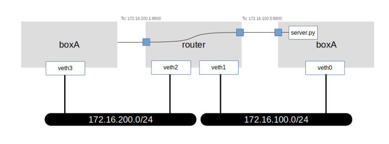
Again, there is a form of NATing that can help – destination NATing. Here, we leave the source IP address of the incoming packet as it is, but instead change the destination IP address. Thus, when a request comes in for port 8800 of the router, we change the target IP address to the IP address of boxA. When we do this in the PREROUTING chain, before a routing decision has been taken, the kernel will recognize that the new IP destination address is not a local address and will forward the packet to boxA.

To try this out, we first need a web server. I have put together a simple WSGI based web server, which will be present in the directory lab13 if you have cloned the corresponding repository. In a separate window, start the web server, making it run in the namespace of boxA.

cd lab13
sudo ip netns exec boxA python3 server.py

Now let us add a destination NATing rule to our router. As mentioned before, the change of the destination address needs to take place before the routing decision is taken, i.e. in the PREROUTING chain.

sudo ip netns exec router \
  iptables -t nat -A PREROUTING \
  -p tcp \
  -i veth2 \
  --destination-port 8800 \
  -j DNAT \
  --to-destination 172.16.100.5:8800

In addition, we need to ACCEPT traffic to this new destination in the FORWARD chain.

sudo ip netns exec router \
  iptables -t filter -A FORWARD \
  -p tcp \
  -i veth2 \
  --destination-port 8800 \
  -d 172.16.100.5 \
  -j ACCEPT

Let us now try to reach our web server from boxB.

sudo ip netns exec boxB \
  curl -w "\n" 172.16.200.1:8800

You should now see a short output (a HTML document with “Hello!” in it) from our web server, indicating that the connection worked. Effectively, we have “peeked a hole” into our firewall, connecting port 8080 of the public network front of our router to port 8800 of boxA. Of course, we could also use any other combination of ports, i.e. instead of mapping 8800 to itself, we could as well map port 80 to 8800 so that we could reach our web server on the public IP address of the router on the standard port.

Of course there is much more that we could say about iptables, but this discussion of the core features should put you in a position to read and interpret most iptable rule sets that you are likely to encounter when working with virtual networks, cloud technology and containers. I highly recommend to browse the references below to learn more, and to look at those chains on your local machine that Docker and libvirt install to get an idea how this is used in practice.

References

The Netfilter How-to
The iptables man page
The excellent book Understanding Linux kernel network internals by C.
Benvenuti
The netfilter packet flow

Virtual networking labs – using OpenFlow

In the last few posts, we have already touched on the OpenFlow protocol that plays a central role in most SDNs. Today, we will learn more on OpenFlow and again use Open vSwitch to see the protocol in action.

OpenFlow – the basics

Recall from our previous post that OpenFlow is a protocol that the control plane and the data plane of an SDN use to exchange rules that determine the flow of packets through the (virtual or physical) infrastructure. The standard is maintained by the Open Networking Foundation and is available here.

Let us first try to understand some basic terms. First, the specification describes the behavior of a switch. Logically, the switch is decomposed into two components. There is the control channel which is the part of the switch that communicates with the OpenFlow controller, and there is the datapath which consists of tables defining the flow of packets through the switch and the ports.

The switch maintains two sets of tables that are specified by OpenFlow. First, there are flow tables that contain – surprise – flows, and then, there are group tables. Let us discuss flow tables first.

An entry in a flow table (a flow entry or flow for short) is very similar to a firewall rule in e.g. iptables. It consists of the following parts.

A set of match fields that are used to see which flow entry applies to which Ethernet packet
An action that is executed on a match
A set of counters
Priorities that apply if a packet matches more than one flow entry
Additional control fields like timeouts, flag or cookies that are passed through

Flow tables can be chained in a pipeline. When a packet comes in, the flow tables in the pipeline are processed in sequence. Depending on the action of a matching flow table entry, a packet can then be sent directly to an outgoing port, or be forwarded to the next table in the pipeline for further processing (using the goto-table action). Optionally, a pipeline can be divided into three parts – ingress tables, group tables (more on this later) and egress tables.

A table typically contains one entry with priority zero (i.e. the lowest priority) and no match fields. As non-existing match fields are considered as wildcards, this flow matches all packets that are not consumed by other, more specific flows. Therefore, this entry is called the table-miss entry and determines how packets with no other matching role are handled. Often, the action associated with this entry is to forward the packet to a controller to handle it. If not even a table-miss entry exists in the first table, the packet is dropped.

While the packet traverses the pipeline, an action set is maintained. Each flow entry can add an action to the set or remove an action or run a specific action immediately. If a flow entry does not forward the packet to the next table, all actions which are present in the action set will be executed.

The exact set of actions depends on the implementation as there are many optional actions in the specification. Typical actions are forwarding a packet to another table, sending a packet to an output port, adding or removing VLAN tags, or setting specific fields in the packet headers.

In addition to flow tables, an OpenFlow compliant switch also maintains a group table. An entry in the group table is a bit like a subroutine, it does not contain any matching criteria, but packets can be forwarded to a group by a flow entry. A group contains one or more buckets each of which in turn contains a set of actions. When a packet is processed by a group table entry, a copy will be created for each bucket, and to each copy the actions in the respective bucket will be applied. Group tables have been added with version 1.1 of the specification.

Lab13: seeing OpenFlow in action

After all this theory, it is time to see OpenFlow in action. For that purpose, we will use the setup in lab11, as shown below.

Let us bring up this scenario again.

git clone https://github.com/christianb93/networking-samples
cd networking-samples/lab11
vagrant up

OVS comes with an OpenFlow client ovs-ofctl that we can use to inspect and change the flows. Let us use this to display the initial content of the flow tables. On boxA, run

sudo ovs-vsctl set bridge myBridge protocols=OpenFlow14
sudo ovs-ofctl -O OpenFlow 14 show myBridge

The first command instructs the bridge to use version 1.4 of the OpenFlow protocol (by default, an OVS bridge still uses the rather outdated version 1.0). The second command asks the CLI to provide some information on the bridge itself and the ports. Note that the bridge has a datapath id (dpid) which is identical to the datapath ID stored in the Bridge OVSDB table (use ovs-vsctl list Bridge to verify this). For this and for all commands, we use the switch -O to make sure that the client uses version 1.4 of the protocol as well. As an example, here is the command to display the flow table.

sudo ovs-ofctl -O OpenFlow14 dump-flows myBridge

This should create only one line of output, describing a flow in table 0 (the first table in the pipeline) with priority 0 and no match fields. This is the table-miss rule mentioned above. The associated action NORMAL specifies that the normal switch processing should take place, i.e. the device should operate like an ordinary switch without involving OpenFlow.

Now let us generate some traffic. Open an SSH connection to to box B and execute

sudo docker exec -it web3 /bin/bash
ping -i 1 -c 10 172.16.0.1

to create 10 ICMP packets. If we now take another look at the OpenFlow table, we should see that the counter n_packets has changed and should now be 24 (10 ICMP requests, 10 ICMP replies, 2 ARP requests and 2 ARP replies).

Next, we will add a flow which will drop all traffic with TCP target port 80 coming in from the container web3. Here is the command to do this.

sudo ovs-ofctl \
     -O OpenFlow14 \
     add-flow \
      myBridge  \
     'table=0,priority=1000,           
      eth_type=0x0800,ip_proto=6,tcp_dst=80,action='

The syntax of the match fields and the rules is a bit involved and described in more detail in the man-pages for ovs-actions and ovs-fields. Note that we do not specify an action, which implies that the packet will be dropped. When you display the flow tables again, you will see the additional rule being added.

Now head over into the terminal connected to the container web3 and try to curl web1. You should see an error message from curl telling you that the destination could not be reached. If you dump the flows once more, you will find that the statistic of our newly added rule have changed and the counter n_packets is now 2. If we delete the flow again using

sudo ovs-ofctl \
     -O OpenFlow14 \
     del-flows \
     myBridge \
     'table=0,eth_type=0x0800,ip_proto=6,tcp_dst=80'

and repeat the curl, it should work again.

This was of course a simple setup, with only one table and no group tables. Much more complex processing can be realized with OpenFlow, and we refer to the OVS tutorials to see some examples in action.

One final note which might be useful when it comes to debugging. OVS is – as many switches – not a pure OpenFlow switch, but in addition to the OpenFlow tables maintains another set of rules called the datapath flow. Sometimes, this causes confusion when the observed results do not seem to match the existing OpenFlow table entries. These additional flows can be dumped using the ovs-appctl tool, see the Open vSwitch FAQs for details.

Virtual networking labs – Open vSwitch in practice

In the last post, we have discussed the architecture of Open vSwitch and how it with a control plane to realize an SDN. Today, we will make this a bit more tangible by running two hands-on labs with OVS.

The labs in this post are modelled after some of the How-to documents that are part of the Open vSwitch documentation, but use a combination of virtual machines and Docker to avoid the need for more than one physical machine. In both labs, we bring up two virtual machines which are connected via a VirtualBox virtual network, and inside each machine, we bring up two Docker containers that will eventually interact via OVS bridges.

Lab 11: setting up an overlay network with Open vSwitch

In the first lab, we will establish interaction between the OVS bridges on the two involved virtual machines using an overlay network. Specifically, the Docker containers on each VM will be connected to an OVS bridge, and the OVS bridges will use VXLAN to talk to each other, so that effectively, all Docker containers appear to be connected to an Ethernet network spanning the two virtual machines.

Instead of going through all steps required to set this up, we will again bring up the machines automatically using a combination of Vagrant and Ansible, and then discuss the major steps and the resulting setups. To run the lab, you will again have to download the code from my repository and start Vagrant.

git clone https://github.com/christianb93/networking-samples
cd lab11
vagrant up

While this is running, let us quickly discuss what the scripts are doing. First, of course, we create two virtual machines, each running Ubuntu Bionic. In each machine, we install Open vSwitch and Docker. We then install the docker Python3 module to make Ansible happy.

Next, we bring up two Docker containers, each running an image which is based on NGINX but has some networking tools installed on top. For each container, we set up a pair of two VETH devices. One of the devices is then moved into the networking namespace of the container, and one of the two devices will later be added to our bridge, so that these VETH device pairs effectively operate like an Ethernet cable connecting the containers to the bridge.

We then create the OVS bridge. In the Ansible script, we use the Ansible OVS module to do this, but if you wanted to create the bridge manually, you would use a command like

ovs-vsctl add-br myBridge \
           -- add-port myBridge web1_veth1 \
           -- add-port myBridge web2_veth1

This is actually a combination of three commands (i.e updates on the OVSDB database) which will be run in one single transaction (the OVS CLI uses the double dashes to combine commands into one transaction). With the first part of the command, we create a virtual OVS bridge called myBridge. With the second and third line, we then add two ports, connected to the two VETH pairs that we have created earlier.

Once the bridge exists and is connected to the containers, we add a third port, which is a VLXAN port, which, using a manual setup, would be the result of the following commands.

ovs-vsctl add-port myBridge vxlan0 \\
          -- set interface vxlan0 type=vxlan options:remote_ip=192.168.50.4  options:dst_port=4789 options:ttl=5

Again, we atomically add the port to the bridge and pass the VXLAN options. We set up the VTEP as a point-to-point connection to the second virtual machine, using the standard UDP port and a TTL of five to avoid that UDP packets get lost.

Finally, we configure the various devices and assign IP addresses. To configure the devices in the container namespaces, we could attach to the containers, but it is easier to use netns to run the required commands within the container namespaces.

Once the setup is complete, we are ready to explore the newly created machines. First, use vagrant ssh boxA to log into boxA. From there, use Docker exec to attach to the first container.

sudo docker exec -it web1 "/bin/bash"

You should now be able to ping all other containers, using the IP addresses 172.16.0.2 – 172.16.0.4. If you run arp -n inside the container, you will also find that all three IP addresses are directly resolved into MAC addresses and are actually present on the same Ethernet segment.

To inspect the bridges that OVS has created, exit the container again so that we are now back in the SSH session on boxA and use the command line utility ovs-vsctl to list all bridges.

sudo ovs-vsctl list-br

This will show us one bridge called myBridge, as expected. To get more information, run

sudo ovs-vsctl show

This will print out the full configuration of the current OVS node. The output should look similar to the following snippet.

af3a2230-3d2a-4364-a0b9-1da4e32211e4
    Bridge myBridge
        Port "web2_veth1"
            Interface "web2_veth1"
        Port "vxlan0"
            Interface "vxlan0"
                type: vxlan
                options: {dst_port="4789", remote_ip="192.168.50.5", ttl="5"}
        Port "web1_veth1"
            Interface "web1_veth1"
        Port myBridge
            Interface myBridge
                type: internal
    ovs_version: "2.9.2"

We can see that the output nicely reflects the structure of our network. There is one bridge, with three ports – the two VETH ports and the VXLAN port. We also see the parameters of the VXLAN ports that we have specified during creation. It is also possible to obtain the content of the OVSDB tables that correspond to the various objects in JSON format.

sudo ovs-vsctl list bridge
sudo ovs-vsctl list port
sudo ovs-vsctl list interface

Lab 12: VLAN separation with Open vSwitch

In this lab, we will use a setup which is very similar to the previous one, but with the difference that we use layer 2 technology to span our network across the two virtual machines. Specifically, we establish two VLANs with ids 100 (containing web1 and web3) and 200 (containing the other two containers). On those two logical Ethernet networks, we establish two different layer 3 networks – 192.168.50.0/24 and 192.168.60.0/24.

The first part of the setup – bringing up the containers and creating the VETH pairs – is very similar to the previous labs. Once this is done, we again set up the two bridges. On boxA, this would be done with the following sequence of commands.

sudo ovs-vsctl add-br myBridge
sudo ovs-vsctl add-port myBridge enp0s8
sudo ovs-vsctl add-port myBridge web1_veth1 tag=100
sudo ovs-vsctl add-port myBridge web2_veth1 tag=200

This will create a new bridge and first add the VM interface enp0s8 to it. Note that by default, every port added to OVS is a trunk port, i.e. the traffic will carry VLAN tags. We then add the two VETH ports with the additional parameter tag which will mark the port as an access port and define the corresponding VLAN ID.

Next we need to fix our IP setup. We need to remove the IP address from the enp0s8 as this is now part of our bridge, and set the IP address for the two VETH devices inside the containers.

sudo ip addr del 192.168.50.4 dev enp0s8
web1PID=$(sudo docker inspect --format='{{.State.Pid}}' web1)
sudo nsenter -t $web1PID -n ip addr add  192.168.50.1/24 dev web1_veth0
web2PID=$(sudo docker inspect --format='{{.State.Pid}}' web2)
sudo nsenter -t $web2PID -n ip addr add  192.168.60.2/24 dev web2_veth0

Finally, we need to bring up the devices.

sudo nsenter -t $web1PID -n ip link set  web1_veth0 up
sudo nsenter -t $web2PID -n ip link set  web2_veth0 up
sudo ip link set web1_veth1 up
sudo ip link set web2_veth1 up

The setup of boxB proceeds along the following lines. In the lab, we again use Ansible scripts to do all this, but if you wanted to do it manually, you would have to run the following on boxB.

sudo ovs-vsctl add-br myBridge
sudo ovs-vsctl add-port myBridge enp0s8
sudo ovs-vsctl add-port myBridge web3_veth1 tag=100
sudo ovs-vsctl add-port myBridge web4_veth1 tag=200
sudo ip addr del 192.168.50.5 dev enp0s8
web3PID=$(sudo docker inspect --format='{{.State.Pid}}' web3)
sudo nsenter -t $web3PID -n ip addr add  192.168.50.3/24 dev web3_veth0
web4PID=$(sudo docker inspect --format='{{.State.Pid}}' web4)
sudo nsenter -t $web4PID -n ip addr add  192.168.60.4/24 dev web4_veth0
sudo nsenter -t $web3PID -n ip link set  web3_veth0 up
sudo nsenter -t $web4PID -n ip link set  web4_veth0 up
sudo ip link set web3_veth1 up
sudo ip link set web4_veth1 up

Instead of manually setting up the machines, I have of course again composed a couple of Ansible scripts to do all this. To try this out, run

git clone https://github.com/christianb93/networking-samples
cd lab12
vagrant up

Now log into one of the boxes, say boxA, attach to the web1 container and try to ping web3 and web4.

vagrant ssh boxA
sudo docker exec -it web1 /bin/bash
ping 192.168.50.3
ping 192.168.60.4

You should see that you can get a connection to web3, but not to web4. This is of course what we expect, as the VLAN tagging is supposed to separate the two networks. To see the VLAN tags, open a second session on boxA and enter

sudo tcpdump -e -i enp0s8

When you now repeat the ping, you should see that the traffic generated from within the container web1 carries the VLAN tag 100. This is because the port to which enp0s8 is attached has been set up as a trunk port. If you stop the dump and start it again, but this time listening on the device web1_veth1 which we have added to the bridge as an access port, you should see that no VLAN tag is present. Thus the bridge operates as expected by adding the VLAN tag according to the tag of the access port on which the traffic comes in.

In the next post, we will start to explore another important feagure of OVS – controlling traffic using flows.

Virtual networking labs – a short introduction to Open vSwitch

In the previous posts, we have used standard Linux tools to establish and configure our network interfaces. This is nice, but becomes very difficult to manage if you need to run environments with hundreds or even thousands of machines. Open vSwitch (OVS) is an Open source software switch which can be integrated with SDN control planes and cloud management software. In this post, we will look a bit at the theoretical background of OVS, leaving the practical implementation of some examples to the next post.

Some terms from the world of software defined networks

It is likely that you have heard the magical word SDN before, and it is also quite likely that you have already found that giving a precise meaning to this term is hard. Still, there is a certain agreement that one of the core ideas of SDN is to separate data flow through your networking devices from the and networking configuration.

In a traditional data center, your network would be implemented by a large number of devices like switches and routers. Each of these devices holds some configuration and typically has a way to change that configuration remotely. Thus, the configuration is tightly integrated with the networking infrastructure, and making sure that the entire configuration is consistent and matches the desired state of your network is hard.

With sofware defined networking, you separate the configuration from the networking equipment and manage it centrally. Thus, the networking equipment handles the flow of data – and is referred to as the data plane or flow plane – while a central component called the control plane is responsible for controlling the flow of data.

This is still a bit vague, but becomes a bit more tangible when we look at an example. Enter Open vSwitch (OVS). OVS is a software switch that turns a Linux server (which we will call a node) into a switch. Technically, OVS is a set of server processes that are installed on each node and that handle the network flow between the interfaces of the node. These nodes together make up the data plane. On top of that, there is a control plane or controller. This controller talks to the individual nodes to make sure the rules that they use to manage traffic (called the flows) are set up accordingly.

To allow controllers and switch nodes to interact, an open standard called OpenFlow has been created which defines a common way to describe flows and to exchange data between the controller and the switches. OVS supports OpenFlow (currently only version 1.1 is supported) and thus can be combined with OpenFlow based controllers like Faucet or Open Daylight, creating a layered architecture as follows. Additionally, a switch can be configured to ask the controller how to handle a packet for which no matching flow can be found.

Here, OVS uses OpenFlow to exchange flows with the controller. To exchange information on the underlying configuration of the virtual bridge (which ports are connected, how are these ports set up, …) OVS provides a second protocol called OVSDB (see below) which can also be used by the control plane to change the configuration of the virtual switch (some people would probably prefer to call the part of the control logic which handles this the management plane in contrast to the control plane, which really handles the data flow only).

Components of Open vSwitch

Let us now dig a little bit into the architecture of OVS itself. Essentially, OVS consists of three components plus a set of command-line interfaces to operate the OVS infrastructure.

First, there is the OVS virtual switch daemon ovs-vswitchd. This is a server process running on the virtual switch and is connected to a socket (usually a Unix socket, unless it needs to communicate with controllers not on the same machine). This component is responsible for actually operating the software defined switch.

Then, there is a state store, in the form of the ovsdb-server process. This process is maintaining the state that is managed by OVS, i.e. the objects like bridges, ports and interfaces that make up the virtual switch, and tables like the flow tables used by OVS. This state is usually kept in a file in JSON format in /etc/openvswitch. The OVSDB connects to the same Unix domain socket as the Switch daemon and uses it to exchange information with the Switch daemon (in the database world, the switch daemon is a client to the OVSDB database server). Other clients can connect to the OVSDB using a JSON based protocol called the OVSDB protocol (which is described in RFC 7047) to retrieve and update information.

The third main component of OVS is a Linux kernel module openvswitch. This module is now part of the official Linux kernel tree and therefore is typically pre-installed. This kernel module handles one part of the OVS data path, sometimes called the fast path. Known flows are handled entirely in kernel space. New flows are handled once in the user space part of the datapath (slow path) and then, once the flow is known, subsequently in the kernel data path.

Finally, there are various command-line interfaces, the most important one being ovs-vsctl. This utility can be used to add, modify and delete the switch components managed by OVS like bridges, port and so forth – more on this below. In fact, this utility operates by making updates to the OVSDB, which are then detected and realized by the OVS switch daemon. So the OVSDB is the leading provider of the target state of the system.

The OVS data model

To understand how OVS operates, it is instructive to look at the data model that describes the virtual switches deployed by OVS. This model is verbally described in the man pages. If you have access to a server on which OVS is installed, you can also get a JSON representation of the data model by running

ovsdb-client get-schema Open_vSwitch

At the top level of the hierarchy, there is a table called Open_vSwitch. This table contains a set of configuration items, like the supported interface types or the version of the database being used.

Next, there are bridges. A bridge has one or more ports and is associated with a set of tables, each table representing a protocol that OVS supports to obtain flow information (for instance NetFlow or OpenFlow). Note that the Flow_Table does not contain the actual OpenFlow flow table entries, but just additional configuration items for a flow table. In addition, there are mirror ports which are used to trace and monitor the network traffic (which we ignore in the diagram below).

Each port refers to one or more interfaces. In most situations, each port has one interface, but in case of bonding, for instance, one port is supported by two interfaces. In addition, a port can be associated with QoS settings and queue for traffic control.

Finally, there are controllers and managers. A controller, in OVS terminology, is some external system which talks to OVS via OpenFlow to control the flow of packets through a bridge (and thus is associated with a bridge). A manager, on the other hand, is an external system that uses the OVSDB protocol to read and update the OVSDB. As the OVS switch daemon constantly polls this database for changes, a manager can therefore change the setup, i.e. add or remove bridges, add or remove ports and so on – like a remote version of the ovs-vsctl utility. Therefore, managers are associated with the overall OVS instance.

Installation and first steps with OVS

Before we get into the actual labs in the next post, let us see how OVS can be installed, and let us use OVS to create a simple bridge in order to get used to the command line utilities.

On an Ubuntu distribution, OVS is available as a collection of APT packages. Usually, it should be sufficient to install openvswitch-switch, which will pull in a few additional dependencies. There are similar packages for other Linux distributions.

Once the installation is complete, you should see that two new server processes are running, called (as you might expect from the previous sections) ovsdb-server and ovs-vswitchd. To try out that everything worked, you can now run the ovs-vsctl utility to display the current configuration.

$ ovs-vsctl show
518a2ed6-56d0-433f-98f2-a575daf20f72
    ovs_version: "2.9.2"

The output is still very short, as we have not yet defined any objects. What it shows you is, in fact, an abbreviated version of the one and only entry in the Open_vSwitch table, which shows the unique row identifier (UUID) and the OVS version installed.

Now let us populate the database by creating a bridge, currently without any ports attached to it. Run

sudo ovs-vsctl add-br myBridge

When we now inspect the current state again using ovs-vsctl show, the output should look like this.

518a2ed6-56d0-433f-98f2-a575daf20f72
    Bridge myBridge
        Port myBridge
            Interface myBridge
                type: internal
    ovs_version: "2.9.2"

Note how the output reflects the hierarchical structure of the database. There is one bridge, and attached to this bridge one port (this is the default port which is added to every bridge, similarly to a Linux bridge where creating a bridge also creates a device that has the same name as the bridge). This port has only one interface of type “internal”. If you run ifconfig -a, you will see that OVS has in fact created a Linux networking device myBridge as well. If, however, you run ethtool -i myBridge, you will find that this is not an ordinary bridge, but simply a virtual device managed by the openvswitch driver.

It is interesting to directly inspect the content of the OVSDB. You could either do this by browsing the file /etc/openvswitch/conf.db, or, a bit more conveniently, using the ovsdb-client tool.

sudo ovsdb-client dump Open_vSwitch

This will provide a nicely formatted dump of the current database content. You will see one entry in the Bridge table, representing the new bridge, and corresponding entries in the Port and Interface table.

This closes our post for today. In the next post, we will setup an example (again using Vagrant and Ansible to do all the heavy lifting) in which we connect containers on different virtual machines using OVS bridges and a VXLAN tunnel. In the meantime, you might want to take a look at the following references which I found helpful.

Click to access OpenVSwitch.pdf

https://github.com/openvswitch/ovs
https://tools.ietf.org/html/rfc7047

Virtual networking labs – overlay networks

In the last post, we have looked at virtual networking on the Ethernet level. In modern cloud environments, a second class of virtual networks has gained importance, which uses higher level protocols to tunnel Ethernet frames. These networks are called overlay networks, and we will start to look at them in this post.

VXLAN – the basics

The VLAN technology that we have looked at in the last post is useful, but has some limitations. First, there is the maximum number of possible VLANs (4096). In practice, certain VLAN ranges need to be reserved for internal purposes, further limiting the number of available VLANs. In cloud environments with a large number of tenants, this limit can easily be reached if we try to implement all virtual networks via VLAN. In addition, VLAN tags inserted by the tenants could conflict with the VLAN tags inserted by the host operating systems.

To solve these problems, a new standard called VXLAN was developed a couple of years back, which is described (though not defined, as this is an informational RFC) in RFC 7348. The basic idea of VXLAN is actually quite simple. On each host involved, we create a virtual network device. When an Ethernet frame needs to be transmitted via this device, the host creates a UDP packet, puts the Ethernet frame as payload into this packet and sends it to the target host. The target host receives the packet, strips off the headers, and re-injects the payload (i.e. the original Ethernet frame) into the networking stack of the target system. Thus Ethernet frames travels on top of UDP, and the virtual Ethernet networks logically sits on top of the layer 3 IP network used to exchange the UDP packets, leading to the name overlay network.

To be able to isolate different VXLANs from each other, a 24 bit VXLAN network identifier (VNI) is used. The implementation needs to make sure that Ethernet frames are only delivered within the same VNI, thus isolating the different VXLAN networks from each other. A host that is able to provide VXLAN devices and to participate in the exchange of UDP packets is called a VXLAN tunnel endpoint (VTEP). Thus to send an Ethernet frame over VXLAN, a VTEP needs to

Add a VXLAN header that contains the VNI, so that the receiving VTEP can make sure that the frame is only delivered within the correct VNI
Pass the resulting data as payload to the own IP stack, which will add a UDP, IP and Ethernet header to be able to transmit the frame over an existing layer 2 network

To be able to locate the UDP target address to which we have to send an encapsulated Ethernet frame, each VTEP needs to maintain a table containing mapping between the IP addresses of other VTEPs and the corresponding MAC addresses. A VTEP typically learns how to populate this table and uses IP multicast to ask other VTEPS to resolve unknown MAC addresses, similar to the ARP protocol.

When VXLAN is used, there are a few points that should be kept in mind. First, we do of course add quite a bit of overhead. For every Ethernet frame that is being exchanged, we add a second Ethernet header, an IP header and a UDP header, plus the processing time it takes on the host to travel the networking stack up and down once more. In addition, there is a problem with the MTU (maximum transfer unit) configured for the VXLAN endpoints. As the Ethernet frames on the physical network are longer than the Ethernet frames on the overlay network (as we need the additional headers), we will have to increase the MTU on the physical network to account for this in order to avoid unnecessary fragmentation. Also, using VXLAN implies that your Ethernet frames flow in clear text over the IP connection, so if you want to use VXLAN across unsecure network areas, then you should use some form of encryption like IPSec.

Lab 9: setting up a point-to-point VXLAN connection

To see this in action, let us first implement a very basic scenario. Assume that we have two hosts (virtual machines provided by VirtualBox in our case) that are part of the same layer 3 network. On each host, we ask the Linux kernel to create a virtual device of type VXLAN. To this virtual device, we can assign IP addresses as usual. Any Ethernet frames sent to the device will be encapsulated using the VXLAN protocol and will be sent to the peer, where the Linux kernel will strip off the outer header and re-inject the Ethernet frame. So the Linux kernel acts as a VTEP on both sides.

Again, I have automated the setup using Vagrant and Ansible. To run the example, simply enter the following commands

git clone https://github.com/christianb93/networking-samples
cd networking-samples/lab9
vagrant up

To inspect the setup, let us first SSH into boxA. If you run ifconfig -a, you will in fact see a new device called vxlan0. This device has been created and configured by our Ansible script using the following commands.

ip link add type vxlan id 100 remote 192.168.50.5 dstport 4789 dev enp0s8
ip addr add 192.168.60.4/24 dev vxlan0
ip link set vxlan0 up

The first command creates the device, specifying the VNI 100, the IP address of the peer, the port number to use for the UDP connection (we use the port number defined in RFC 7348) and the physical device to be used for the transmission. The second and third command then assign an IP address and bring the device up.

When you run netstat -a on boxA, you will also find that a UDP socket has been created on port 4789, this socket is ready to accept UDP packets from the peer carrying encapsulated Ethernet frames. The setup on boxB is similar, using of course a different IP address.

Let us now try to exchange traffic and to display the packets that go forth and back. For that purpose, open an SSH session on boxB as well and start a tcdump session listening on vxlan0.

sudo tcpdump -e -i vxlan0

You will a sequence of ARP and IPv4 packets, with the source and target MAC addresses matching the MAC addresses of the vxlan0 devices on the respective hosts. Thus the device acts like an ordinary Ethernet device, as expected.

Now let us change the setup and start to dump traffic on the underlying physical interface.

sudo tcpdump -e -i enp0s8

When you now repeat the ping, you will see that the packets arriving at the physical interface are UDP packets. In fact, tcpdump properly recognizes these frames as VXLAN frames and also prints the inner headers. We see that the outer Ethernet headers contain the MAC addresses of the underlying network interfaces of boxA and boxB, whereas the inner headers contain the MAC addresses of the vxlan0 devices.

Lab 10: VXLAN and IP multicasting

So far, we have used a direct point-to-point connection between the two hosts involved in the VXLAN network. In reality, of course, things are more complicated. Suppose, for instance, that we have three hosts representing VTEP endpoints. If an Ethernet frame on one of the hosts reaches the VXLAN interface, the kernel needs to determine to which of the other hosts the resulting UDP packet should be sent.

Of course, we could simply broadcast the packet to all hosts on the IP network, using a broadcast, but this would be terribly inefficient. Instead, VXLAN uses IP multicast functionality. To this end, the administrator setting up VXLAN needs to associate an IP multicast address with each VNI. A VTEP will then join this group and will use the IP multicast address for all traffic that needs to go to one or more Ethernet destinations. In a local network, you want to use one of the “private” IP multicast groups in the range 239.0.0.0 – 239.255.255.255 reserved by RFC 2365, for instance within the local scope 239.255.0.0/16.

To study this, I have created lab 10 which establishes a scenario in which three hosts serve as VTEP to span a VXLAN with VNI 100. As always, grab the code from GitHub, cd into the directory lab10 and run vagrant up to start the example.

The setup is very similar to the setup for the point-to-point connection above, with the difference that when bringing up the VXLAN device, we have removed the remote parameter and replaced it by the group parameter to tie the VNI to the multicast group.

ip link \
   add type vxlan \
   id 100 \
   group 239.255.0.1 \
   ttl 5 \
   dstport 4789 \
   dev enp0s8

Note the parameter TTL which defines the initial TTL that will be set on the UDP packets sent out by the VTEP. When I tried this setup first, I did not set the TTL, resulting in the default of one. With this setup, however, ARP requests were not answered by the target host, and I had to increase the TTL by adding the additional parameter.

Let us test this setup. Open SSH connections to the boxA and boxB. First, we can use ip maddr show enp0s8 to verify that on both machines, the interface enp0s8 has joined the multicast group 239.255.0.1 that we specified when bringing up the VXLAN. Then, start a tcpdump session on enp0s8 on boxC and ping the VXLAN IP address 192.168.60.5 of boxB from boxA. As this is the first time we establish this connection, the Ethernet device should emit an ARP request. This ARP request is encapsulated and sent out as an IP multicast with IP target address 239.255.0.1. In tcpdump, the corresponding output (again displaying the outer and inner headers) looks as follows.

06:30:44.255166 08:00:27:fe:3b:d0 (oui Unknown) > 01:00:5e:7f:00:01 (oui Unknown), ethertype IPv4 (0x0800), length 92: 192.168.50.4.57732 > 239.255.0.1.4789: VXLAN, flags [I] (0x08), vni 100
b6:02:f0:c8:15:85 (oui Unknown) > Broadcast, ethertype ARP (0x0806), length 42: Request who-has 192.168.60.5 tell 192.168.60.4, length 28

We can clearly see that the outer IP header has the multicast IP address as target address, and that the inner frame is an ARP request, looking to resolve the IP address of the VXLAN device on boxB.

The multicast mechanism is used to initially discover the mapping of IP addresses to Ethernet addresses. However, this is typically only required once, because the VTEP is able to learn this mapping by storing it in a forwarding database (FDB). To see this mapping, switch to boxA and run

bridge fdb show dev vxlan0

In the output, you should be able to locate the Ethernet address of the VXLAN device on boxC, being mapped to the IP address of boxC on the underlying network, i.e. 192.168.50.6.

Virtual networking labs – virtual Ethernet networks with VLAN tags

In the previous posts, we have mainly been looking at virtual networking within one single physical hosts. This is nice, but to build cloud environments, we need to establish virtual networks across several physical hosts. In this post, we will start to look into technologies that make this possible and learn how VLAN tagging supports virtual Ethernet networks.

An introduction to virtual Ethernet networks

Today, essentially every Ethernet network you will come across is a switched network, where every server is more or less directly connected to a switch, and the switches are connected to each other to propagate traffic through your data center. A naive approach would be to use layer 2 switches to combine all Ethernet networks into one large broadcast domain, where every node is connected to every other node by a sequence of switches. This approach, however, creates a very large broadcast domain and is difficult to maintain as changes to the topology need to be done by a physical rearrangement. It might therefore be beneficial to have some way of dividing your physical Ethernet network into two or more logical (“virtual”) networks.

For servers that are connected to the same switch, this can be implemented by an approach known as port-based VLAN. To illustrate the idea, let us look at the following configuration, where four servers are connected to four different ports of one switch.

With this setup, a broadcast issued by one server will reach every other server, and all servers are part of one Ethernet network. To introduce virtualization, we could simply add some logic to the switch to divide the ports into two sets, where forwarding of Ethernet frames is only done within those two sets. If, for instance, we define one set to consist of the two ports connected to server 1 and server 2 (green), and the other consisting of the remaining two ports (red), and configure the switch such that it will only forward frames between ports with the same color, we will effectively have established two virtual networks.

This is nice, as – if your switch supports it – no additional hardware is required and you can define and change the configuration entirely in software. But there is a problem. Typically, your data center will have more than one switch. How can you extend these virtual networks across multiple switches? Of course, you could add an additional connection for every virtual network between any two switches, but this will blow up your hardware requirements and again make changes in hardware necessary. To avoid this, a technology called VLAN trunking is needed.

With VLAN trunking, different virtual LANs (VLANs) can share the same physical connection. To enable this, Ethernet frames that travel on this shared part of your infrastructure are enhanced by adding a VLAN tag which contains a numerical ID identifying the VLAN to which they belong, as indicated in the following diagram.

Here, we have two switches, which both use port-based virtual networks as just discussed. The upper two ports of each switch belong to the green network which is assigned the ID 1 (VLAN ID or VID, note that in reality, this ID is often reserved) and the other set of ports is part of VLAN 2 (the red network). When a frame leaves, for instance, the server in the upper left corner and needs to be forwarded to the server in the upper right corner, the switch will add a VLAN tag to indicate that this frame is part of VLAN 1. Then the frame travels across the connection between the two switches. Then the switch on the right hand side receives the frame, it strips off the VLAN frame again and, based on the tag, injects the frame back into its own VLAN 1, so that it can only reach the green ports on the right hand side.

Thus your network is divided into two parts. In the middle, on the connection between the two switches, frames carry the VLAN tag to flag them as being part of the red or green network. Thus the ports facing this part need to be aware of the VLAN tag – these ports are often called trunk ports. The parts of the network behind the switches, however, do never see a VLAN tag, as it is added and removed by the switches when transmitting and receiving on trunk ports. These ports are called access ports. Thus the servers do not need to known to which VLAN they belong, and the configuration can be done entirely on the switches and in software.

The standard that describes all this and also defines how a VLAN tag is added to an Ethernet frame is called IEEE 802.1Q. This standard adds a 16-bit field called TCI – tag control information to the layout of an Ethernet frame. Four bits of this field are reserved for other purposes, so that 12 bits remain for the VLAN ID, allowing a maximum of 4096 different VLANs.

Lab 8: VLAN networking with Linux

Linux has the capability to create virtual Ethernet devices that are associated with a VLAN network. To see this in action, get lab 8 from my GitHub repository and run it.

git clone https://github.com/christianb93/networking-samples
cd networking-samples/lab8
vagrant up

The Vagrantfile and the three Ansible playbooks that are located in this directory will now execute and bring up three virtual machines. Here is a diagram summarizing the network configuration that the scripts create (we will see how this is done manually further below).

We see that all three machines are connected to one virtual Ethernet cable (we use a VirtualBox internal network for that purpose). The three interfaces attached to this network are configured as part of the IP network 192.168.50.0/24.

However, in addition, we have set up two virtual networks – one network with VLAN ID 100 (green), and a second network with VLAN ID 200 (red). In each Linux machine, the virtual networks to which the machine is attached is represented by a virtual device called a VLAN device.

Let us look at boxA to see how this works. On boxA, the Ansible playbook that got executed during the vagrant up did run the following command

vconfig add enp0s8 100

This command is creating a new network interface enp0s8.100 sitting on top of enp0s8 but being associated with the VID 100. This device is an ordinary device from the point of view of the operating system, i.e. you can assign IP addresses, add routes and so forth.

Such a VLAN device operates as follows. When an Ethernet frame arrives on the underlying device, enp0s8 in our case, the kernel checks whether the frame contains a VLAN tag. If no, the processing is as usual. If yes, then the kernel next checks whether a VLAN device is associated with this VID. If there is one, it strips off the VLAN tag, changes the frame so that it appears to be coming from the virtual VLAN device and re-injects the frame into the networking stack. The frame then travels up the stack and can be processed by the higher layers, e.g. the IP layer. Conversely, if a frame needs to be transmitted on enp0s8.100, the kernel adds a VLAN tag with the VID 100 to the frame and redirects it to the physical device enp0s8.

Let us see this in action. Open two SSH connections, one to boxA, and one to boxB – if you use the Gnome terminal, simply run

for i in "A" "B" ; do gnome-terminal -e "vagrant ssh box$i"; done

In boxA, start a tcpdump session on the VLAN device.

sudo tcpdump -e -i enp0s8.100

On boxB, ping boxA, using the IP address 192.168.60.4 (the IP address of the VLAN device). You will see an ordinary frame coming in, with ethertype IPv4. There is no VLAN tag within this frame, and the VLAN device operates like a physical device with no VLAN tagging.

Now, stop the tcpdump session and start it again, but this time, use enp0s8 instead of enp0s8.100, i.e. the underlying physical device. If you now run a ping again, you will see that the ethertype of the incoming packages has changed and is now 802.1Q, indicating that the frame is tagged (tcpdump will also show you the VLAN ID 100).

When you ping boxA from boxB using the IP address 192.168.50.4, the traffic will be as expected, coming in on enp0s8 without any VLAN tag, and will not reach enp0s8.100. Thus even though you have put a VLAN device on top of the physical interface, you can still use the physical interface as usual.

It is instructive to check the ARP cache on boxB using arp -n after the pings have been exchanged. You will see that the MAC address of the enp0s8 device on boxA now appears twice, once with the IP address 192.168.50.4 and once with 192.168.60.4. So the MAC address is shared between the virtual VLAN device and the physical device.

Still, the traffic is separated by the Linux kernel. If, for instance, you try to ping 192.168.70.6 (one of the IP addresses of boxC) from boxA, you will not be successful, because this IP address is on the red network and not reachable from the green network. If you run the ping on boxB, however, it will work, because boxB participates in both virtual networks.

This closes todays lab. In the next lab, we will start to look at a completely different approach to building virtual networks – overlay networks.

Using Ansible with a jump host

For an OpenStack project using Ansible, I recently had to figure out how to make Ansible work with a jump host. After an initial phase of total confusion, I finally found my way through the documentation and various sources and ended up with several working configurations. This post documents what I have learned on that journey to hopefully make your life a bit easier.

Setup

In my previous posts on Ansible, I have used a rather artificial setup – a set of hosts which all expose the SSH port on the network so that we can connect directly. In real world, hosts are often hidden behind firewalls, and a pattern that you will see frequently is that only one host in a network can directly be reached via SSH – called a jump host or a bastion host – and you need to SSH into all the other hosts from there.

To be able to experiment with this situation, let us first create a lab environment which simulates this setup on Google’s cloud plattform (but any other cloud platform that has a concept of a VPC should do as well).

First, we need a project in which our resources will live. For this lab, create a new project called terraform-project with a project ID like terraform-project-12345 (of course, you will not be able to use the exact same project ID as I did, as project IDs are supposed to be unique), for instance from the Google Cloud console under “Manage Resources” in the IAM & Admin tab.

Next, create a service account for this project and assign the role “Compute Admin” to this account (which is definitely not the most secure setup and clearly not advisable for a production setup). Create a key for this service account, download the key in JSON format and store it as ~/gcp_terraform_service_account.json

In addition, you will need a private / public SSH key pair. You can reuse an existing key or create a new one using

ssh-keygen -P "" -b 2048 -t rsa -f ~/.ssh/gcp-default-key

Now we are ready to download and run the Terraform script. To do this, open a terminal on your local PC and enter

git clone https://github.com/christianb93/ansible-samples
cd ansible-samples/jumphost
terraform init
terraform apply -auto-approve

When opening the Google Cloud Console after the script has completed, you should be able to verify that two virtual networks with two machines on them have been created, with a topology as summarized by the following diagram.

So we see that there is a target host which is connected to a private network only, and a jump host which has a public IP address and is attached to a public network.

One more hint: when playing with SSH, keep in mind that on the Ubuntu images used by GCE, sshguard is installed by default which will monitor the SSH log files and, if something that looks like an attach is identified, insert a firewall rule into the filter table which blocks all incoming traffic (including ICMP)from the machine from which the suspicious SSH connections came. As playing around with some SSH features might trigger an alert, the Terraform setup script will therefore remove sshguard from the machines upon startup (though there would of course be smarter ways to deal with that, for instance by adding our own IP to the sshguard whitelist).

The SSH ProxyCommand feature

Before talking about SSH and jump hosts, we first have to understand some features of SSH (and when I say SSH here and in the following, I mean OpenSSH) that are relevant for such a configuration. Let us start with the ProxyCommand feature.

In an ordinary setup, SSH will connect to an SSH server via TCP, i.e. it will establish a TCP connection to port 22 of the server and will start to run the SSH protocol over this connection. You can, however, tell SSH to operate differently. In fact, SSH can spawn a process and write to STDIN of that process instead of writing to a TCP connection, and similarly read from STDOUT of this process. Thus we replace the TCP connection as communication channel by an indirect communication via this proxy process. In general, it is assumed that the proxy process in turn will talk to an SSH server in the background. The ProxyCommand flag tells SSH to use a proxy process to communicate with a server instead of a TCP connection and also how to start this process. Here is a diagram displaying the ordinary connection method (1) compared to the use of a proxy process (2).

To see this feature in action, let us play a bit with this and netcat. Netcat is an extremely useful tool which can establish a connection to a socket or listen on a socket, send its own input to this socket and print out whatever it sees on the socket.

Let us now open a terminal and run the command

nc -l 1234

which will ask netcat to listen for incoming connections on port 1234. In a second terminal windows, run

ssh -vvv \
    -o "ProxyCommand nc localhost 1234" \
    test@172.0.0.1

Here the IP address at the end can be any IP address (in fact, SSH will not even try to establish a connection to this IP as it uses the proxy process to communicate with the apparent server). The flag -vvv has nothing to do with the proxy, but just produces some more output to better see what is going on. Finally, the ProxyCommand flag will specify to use nc localhost 1234 as proxy process, i.e. an instance of netcat connecting to port 1234 (and thus to the instance of netcat in our second terminal).

When you run this, you should see a string similar to

SSH-2.0-OpenSSH_7.6p1 Ubuntu-4

on the screen in the second terminal, and in the first terminal, SSH will seem to wait for something. Copy this string and insert it again in the second terminal (in which netcat is running) below this output. At this point, some additional output should appear, starting with some binary garbage and then printing a few strings that seem to be key types.

This is confusing, but actually expected – let us try to understand why. When we start the SSH client, it will first launch the proxy process, i.e. an instance of netcat – let us call this nc1. This netcat instance receives 1234 as the only parameter, so it will happily try to establish a connection to port 1234. As our second netcat instance – which we call nc2 – is listening on this port, it will connect to nc2.

From the clients point of view, the channel to the SSH server is now established, and the protocol version exchange as described in section 4.2 of RFC4253 starts. Thus the client sends a version string – the string you see appearing first in the second terminal – to its communication channel. In our case, this is STDIN of the proxy process nc1, which takes that string and sends it to nc2, which in turn prints it on the screen.

The SSH client is now waiting for the servers version string as the response. When we copied that string to the second terminal, we provided it as input to nc2, which in turn did send it to nc1 where it was printed on STDOUT of nc1. This data is seen as coming across the communication channel by the SSH client, i.e. from our fictitious SSH server. The client is happy and continues with the next phase of the protocol – the key exchange (KEX) phase described in section 7 of the RFC. Thus the client sends a list of key types that it supports, in the packet format specified in section 6, and this is the garbage followed by some strings that we see. Nice…

STDIO forwarding with SSH

Let us now continue to study a second feature of OpenSSH called standard input and output tunneling which is activated with the -W switch.

The man page is a bit short at this point, stating that this switch requests that standard input and output on the client be forwarded to host on port over the secure channel. Let us try to make this a bit clearer.

First, when you start the SSH client, it will, like any interactive process, connect its STDOUT and STDIN file descriptors to the terminal. When you use the option -W, no command will be executed on the SSH server, but instead the connection will remain open and SSH will establish a connection from the SSH server to a remote host and port that you specify along with the -W switch. Then any input that you provide to the SSH client will travel across the SSH connection and be fed into that connection, whereas anything that is received from this connection from the remote host is sent back via the SSH connection to the client – a bit like a remote version of netcat.

Again, let us try this out. To do this, we need some host and port combination that we can use with -W which will provide some meaningful output. I have decided to use httpbin.org which, among other things, will give you back your own IP address. Let us first try this locally. We will use the shell’s built-in printf statement to prepare a HTTP GET request and feed that into netcat which will connect to httpbin.org, send our request and read the response.

$ printf "GET /ip HTTP/1.0\r\n\r\n" | nc httpbin.org 80
HTTP/1.1 200 OK
Access-Control-Allow-Credentials: true
Access-Control-Allow-Origin: *
Content-Type: application/json
Date: Tue, 17 Dec 2019 18:20:20 GMT
Referrer-Policy: no-referrer-when-downgrade
Server: nginx
X-Content-Type-Options: nosniff
X-Frame-Options: DENY
X-XSS-Protection: 1; mode=block
Content-Length: 45
Connection: Close

{
  "origin": "46.183.103.8, 46.183.103.8"
}

The last part is the actual body data returned with the response, which is our own IP address in JSON format. Now replace our local netcat with its remote version implemented via the SSH -W flag. If you have followed the setup described above, you will have provisioned a remote host in the cloud which we can use as SSH target, and a user called vagrant on that machine. Here is our example code.

$ printf "GET /ip HTTP/1.0\r\n\r\n" | ssh -i ~/.ssh/gcp-default-key -W httpbin.org:80 vagrant@34.89.221.226
HTTP/1.1 200 OK
Access-Control-Allow-Credentials: true
Access-Control-Allow-Origin: *
Content-Type: application/json
Date: Tue, 17 Dec 2019 18:22:17 GMT
Referrer-Policy: no-referrer-when-downgrade
Server: nginx
X-Content-Type-Options: nosniff
X-Frame-Options: DENY
X-XSS-Protection: 1; mode=block
Content-Length: 47
Connection: Close

{
  "origin": "34.89.221.226, 34.89.221.226"
}

Of course, you will have to replace 34.89.221.226 with the public IP address of your cloud instance, and ~/.ssh/gcp-default-key with your private SSH key for this host. We see that this time, the IP address of the host is displayed. What happens is that SSH makes a connection to this host, and the SSH server on the host in turn reaches out to httpbin.org, opens a connection on port 80, sends the string received via the SSH client’s STDIN to the server, gets the response back and sends it back over the SSH connection to the client where it is finally displayed.

TCP/IP tunneling with SSH

Instead of tunneling stdinput / stdoutput through an SSH connection, SSH can also tunnel a TCP/IP connection using the flag -L. In this mode, you specify a local port, a remote host (reachable from the SSH server) and a remote port. The SSH daemon on the server will then establish a connection to the remote host and remote port, and the SSH client will listen on the local port. If a connection is made to the local port, the connection will be forwarded through the SSH tunnel to the remote host.

There is a very similar switch -R which establishes the same mechanism, but with the role of client and server exchanged. Thus the client will connect to the specified target host and port, and the server will listen on a local port on the server. Incoming connections to this port will then be forwarded via the tunnel to the connection held by the client.

Putting it all together – the five methods to use SSH jump hosts

We now have all the tools in our hands to use jump hosts with SSH. It turns out that these tools can be combined in five different ways to achieve our goal (and there might even be more, if you are only creative enough). Let us go through them one by one.

Method 1

We could, of course, simply place the private SSH key for the target host on the jump host and then use ssh to run ssh on the jump host.

scp -i ~/.ssh/gcp-default-key \
    ~/.ssh/gcp-default-key \
    vagrant@34.89.221.226:/home/vagrant/key-on-jump-host
ssh -t -i ~/.ssh/gcp-default-key \
  vagrant@34.89.221.226 \
    ssh -i key-on-jump-host vagrant@192.168.178.3

You will have to adjust the IP addresses to your setup – 34.89.221.226 is the public IP address of the jump host, and 192.168.178.3 is the IP address under which our target host is reachable from the jump host. Also note the -t flag which is required to make the inner SSH process feel that it is connected to a terminal.

This simple approach works, but has the major disadvantage that is forces you to store the private key on the jump host. This makes your jump host a single point of failure in you security architecture, which is not a good thing as this host is typically exposed at a network edge – not a good idea. In addition, this can quickly undermine any serious attempt to establish a central key management in an organisation. So we are looking for methods that will allow you to keep the private key on the local host.

Method two

To achieve this, there is a method which seems to be the “traditional” approach that can find in most tutorials and that uses a combination of netcat and the ProxyCommand flag. Here is the command that we use.

ssh -i ~/.ssh/gcp-default-key \
   -o "ProxyCommand \
     ssh -i ~/.ssh/gcp-default-key vagrant@34.89.221.226\
     nc %h 22" \
   vagrant@192.168.178.3

Again, you will have to adjust the IP addresses in this example as explained above. When you run this, you should be greeted by a shell prompt on the target host – and we can now understand why this works. SSH will first run the proxy command on the client machine, which in turn will invoke another “inner” SSH client establishing a session to the jump host. In this session, netcat will be started on the jump host and connect to the target host.

We have now established a direct channel from standard input / output of the second SSH client – the proxy process – to port 22 of the target host. Using this channel, the first “outer” SSH client can now proceed, negotiate versions, exchange keys and establish the actual SSH session to the target host.

It is interesting to use ps on the client and the jump host and netstat on the jump host to verify this diagram. On the client, you will see two SSH processes, one with the full command line (the outer client) and a second one, spawned by the first one, representing the proxy command. On the jump host, you will see the netcat process that the SSH daemon sshd has spawned, and the TCP connection to the SSH daemon on the target host established by the netcat process.

There is one more mechanism being used here – the symbol %h in the proxy command is an example for what the man page calls a token – a placeholder which is replaced by SSH at runtime. Here, %h is replaced by the host name to which we connect (in the outer SSH command!), i.e. the name or IP of the target host. Instead of hardcoding the port number 22, we could also use the %p token for the port number.

Method three

This approach still has the disadvantage that it requires the extra netcat process on the jump host. In order to avoid this, we can use the same approach using a stdin / stdout tunnel instead of netcat.

ssh -i ~/.ssh/gcp-default-key \
  -o "ProxyCommand \
    ssh -i ~/.ssh/gcp-default-key -W %h:%p vagrant@34.89.221.226"\
  vagrant@192.168.178.3

When you run this and then inspect processes and connections on the jump host, you will find that the netcat process has gone, and the connection from the jump host to the target is initiated by a (child process of) the SSH daemon running on the jump host.

This method is described in many sources and also in the Ansible FAQs.

Method four

Now let us turn to the fourth method that is available in recent versions of OpenSSH – a new ProxyJump directive that can be used in the SSH configuration. This approach is very convention when working with SSH configuration files, so let us take a closer look at it. Let us create a SSH configuration file (typically this is ~/.ssh/config) with the following content:

Host jump-host
  HostName 34.89.221.226
  IdentityFile ~/.ssh/gcp-default-key
  User vagrant 

Host target-host
  HostName 192.168.178.3
  IdentityFile ~/.ssh/gcp-default-key
  User vagrant 
  ProxyJump jump-host

To test this configuration, simply run

ssh target-host

and you should directly be taken to a prompt on the target host. What actually happens here is that SSH looks up the configuration for the host that you specify on the command line – target-host – in the configuration file. There, it will find the ProxyJump directive, referring to the host jump-host. SSH will follow that reference, retrieve the configuration from this host from the same file and use it to establish the connection.

It is instructive to run ps axf in a second terminal on the client after establishing the connection. The output of this command on my machine contains the following two lines.

  49 tty1     S      0:00  \_ ssh target-host
  50 tty1     S      0:00      \_ ssh -W [192.168.178.3]:22 jump-host

So what happens behind the scenes is that SSH will simply start a a second session to open a stdin/stdout tunnel, as we have done it manually before. Thus the ProxyJump option is nothing but a shortcut for what we have done previously.

The equivalent of the ProxyJump directive in the configuration file is the switch -J on the command line. Using this switch directly without a configuration file does, however, have the disadvantage that it is not possible to specify the SSH key to be used for connecting to the jump host. If you need this, you will have to use the -W option discussed above which will provide the same result.

Method five

Finally, there is another method that we could use – TCP/IP tunneling. On the client, we start a first SSH session that will open a local port with port number 8222 and establish a connection to port 22 of the target host.

ssh -i ~/.ssh/gcp-default-key \
  -L 8222:192.168.178.3:22 \
  vagrant@34.89.221.226

Then, in a second terminal on the client, we use this port as the target for an SSH connection. The connection request will then to through the tunnel and we will actually establish a connection to the target host, not to the local host.

ssh -i ~/.ssh/gcp-default-key \
    -p 8222 \
    -o "HostKeyAlias 192.168.178.3" \
    vagrant@127.0.0.1

Why do we need the additional option HostKeyAlias here? Without this option, SSH will take the target host specified on the command line, i.e. 127.0.0.1, and use this host name to look up the host key in the database of known host keys. However, the host key it actually receives during the attempt to establish a connection is the host key of the target host. Therefore, the keys will not match, and SSH will complain that the host key is not known. The HostKeyAlias 192.168.178.3 instructs SSH to use 192.168.178.3 as the host name for the lookup, and SSH will find the correct key.

Ansible configuration with jump hosts

Let us now discuss the configuration needed in Ansible to make this work. As explained in the Ansible FAQs, Ansible has a configuration parameter ansible_ssh_common_args that can be used to define additional parameters to be added to the SSH command used to connect to a host. In our case, we could set this variable as follows.

ansible_ssh_common_args:  '-o "ProxyCommand ssh -o StrictHostKeyChecking=no -o UserKnownHostsFile=/dev/null -i ~/.ssh/gcp-default-key -W %h:%p vagrant@34.89.221.226"'

Here the first few options are used to avoid issues with unknown or changed SSH keys (you can also set them here for the outer SSH connection if this is not yet done in your ansible.cfg file). There are several options that you have to set this variable. As all variables in Ansible, this is a per-host variable which we could set in the inventory or (as the documentation suggests) in a group_vars folder on the file system.

In my repository, I have created an example that uses the technique explained in an earlier post to build an inventory dynamically by capturing Terraform output. In this inventory, we set the ansible_ssh_common_args variable as above to be able to reach our target host via the jump host. To run the example, follow the initial configuration steps as explained above and then do

git clone https://github.com/christianb93/ansible-samples/
cd ansible-samples/jumphost
terraform init
ansible-playbook site.yaml

This playbook will not do anything except running Terraform (which will create the environment if you have not done this yet), capturing the output, building the inventory and connecting once to each host to verify that they can be reached.

There are many more tunneling features offered by SSH which I have not touched upon in this post – X-forwarding, for instance, or device tunneling which creates tun and tap devices on the local and the remote machine and therefore allows us to easily build a simple VPN solution. You might want to play with the SSH man pages (and your favorite search engine) to find out more on those features. Enjoy!

Virtual networking labs – more on bridges

In the previous post, we have seen how a software-defined Linux bridge can be established and how it transparently connects two Ethernet devices. In this post, we will take a closer look at how to set up and monitor bridges and learn how VirtualBox uses bridges for virtual networking.

Lab 6: setting up and monitoring bridges

For this lab, we will start with the setup of lab 5 that we have gone through in the previous post. If you have destroyed your environments again, the easiest way to get back to the point where we left off is to let Vagrant and Ansible do the work. I have created a Vagrantfile and a set of playbooks to take care of this. So simply do

git clone https://github.com/christianb93/networking-samples
cd lab6
vagrant up

to bring up all machines and configure the network interfaces as in my last post. You can then use vagrant ssh to SSH into one of the three virtual machines.

First, let us go through the steps that we have used to set up boxB, the machine on which the bridge is running. Recall that, after installing the bridge-utils package, we used the following sequence of commands.

sudo brctl addbr myBridge
sudo ifconfig enp0s8 promisc 0.0.0.0
sudo ifconfig enp0s9 promisc 0.0.0.0
sudo brctl addif myBridge enp0s8
sudo brctl addif myBridge enp0s9
sudo ifconfig myBridge up

The first command is easy to understand. It uses the brctl command line utility to actually set up a bridge called myBridge.

Next, we re-configure the two devices that we will turn into bridge ports. As explained in chapter 10 of “Understanding Linux network internals”, if an Ethernet frame is received on an interface which has been added to a bridge, the usual processing of the frame (i.e. passing the frame to all registered layer 3 protocol handlers) is skipped, and the frame is handed over to the bridging code. Therefore, it does not make sense to have an IP address associated with our bridge ports enp0s8 and enp0s9 any more. In addition, we need to set the devices into promiscuous mode, i.e. we need to enable them to receive packets which are not directed towards their own Ethernet address. This becomes clear if you look at our network diagram once more.

If an Ethernet frame is sent out by boxC, directed towards the interface of boxA, it will have the MAC address of this interface as target address in its Ethernet header. Still, it needs to be picked up by the enp0s9 device on boxB so that it can be handed over to the bridge. If we would not put the device into promiscuous mode, it would drop the frame as its target MAC address does not match its own MAC address (strictly speaking, setting the device into promiscuous mode manually is not really needed, as the Linux kernel will do this automatically when we add the port to the bridge, but we do this here explicitly to highlight this point).

Once we have re-configured our two network devices, we add them to the bridge using brctl addif. We finally bring up the bridge using ifconfig.

Let us now look a bit into the details of our bridge. First, recall that a bridge usually operates by learning MAC addresses. For a Linux bridge, this holds as well, and in fact, a Linux bridge maintains a table of known MAC addresses and the ports behind which they are located. To display this table, open an SSH connection to boxB and run

sudo brctl showmacs myBridge

If you look at the output, you will see that the bridge differentiates between local and non-local addresses. A local address is the MAC address of an interface which is attached to the bridge. In our case, these are the two interfaces enp0s9 and enp0s8 that are part of your bridge on boxB. A non-local address is the address of an Ethernet device on the local network which is not directly attached to the bridge. In our example, these are the Ethernet devices enp0s8 on boxA and boxC.

You also see that these entries are ageing, i.e. if no frames related to an interface that the bridge knows are seen for some time, the entry is dropped and recreated if the interface appears again. The reason for this behaviour is to avoid problems if you reconfigure your physical network so that maybe an Ethernet device thas has been part of the network behind port 1 moves into a part of the network which is behind port 2.

You can also monitor the traffic that flows through the bridge. If, for instance, you run a sniffer like tcpdump on box B using

sudo tcpdump -e -i myBridge

and then create some traffic using for instance ping, you will see that the packets cross the Ethernet bridge.

It is also instructive to run a traceroute on boxA targeted towards boxC. If you do this, you will find that there is no hop between the two devices, again confirming that our bridge operates on layer 2 and behaves like a direct connection between boxA and boxC.

Finally, let us quickly discuss the configuration of the bridge itself. If you look at the configuration using ifconfig myBridge, you will see that the bridge has a MAC address itself, which is the lowest MAC address of all devices added to the bridge (but can also be set manually). In fact, we will see in a second that it is also possible to assign an IP address to a bridge!

This is a bit confusing, after all, a bridge is logically simply a direct connection between the two ports, but nothing which can by itself emit and absorb Ethernet frames. However, on Linux, setting up a bridge also creates a “default-port” on the bridge which is handled like any other network device. Technically speaking, the bridge driver is itself a network device driver (implemented here), and you can ask it to transmit frames. I tend to think of the situation as in the following image.

When the Linux kernel asks the bridge to transmit a frame, the bridge code will consult its table of known MAC addresses and send the frame to the correct port. Conversely, if a frame is received by any of the two ports enp0s8 or enp0s9 and forwarded to the bridge, the bridge does not only forward the frame to the correct port depending on the destination address, but also delivers the frame to the higher layers of the Linux networking stack if its Ethernet target address matches the MAC address of the bridge (or any of the local MAC address in the table of known MAC addresses).

Let us try this out. In our configuration so far, we have not been able to reach boxB via the bridged network, and, conversely, we could not reach boxA and boxC from boxB (try a ping to verify this). Let us now assign an IP address to the bridge device itself and add a route. On boxB, run

sudo ifconfig myBridge netmask 255.255.0.0 192.168.70.4

which will automatically add a route as well. Now, our network diagram has changed as follows (note the additional IP address on boxB).

You should now be able to ping boxB (192.168.70.4) from both boxA and boxB and vice versa. This capability allows one to use one Linux host as both an Ethernet bridge and a router at the same time.

Lab 7: bridged networking with VirtualBox

So far, we have used VirtualBox to create virtual machines, and have played with bridges inside these machines. Now we will turn this around and see how conversely, VirtualBox can use bridges to realize virtual networks.

It is tempting to assume that what is called bridged networking in the VirtualBox documentation actually uses bridges. This, however, is no longer the case. Instead, when you define a bridged network with VirtualBox, the vboxnetflt netfilter driver that also featured in our last post will be used to attach a “virtual Ethernet cable” to an existing device, and the device will be set into promiscuous mode so that it can pick up Ethernet frames targeted towards the virtual ethernet card of the VM and redirect them to the VirtualBox networking engine. Effectively, this exposes the virtual device of the VM to the local network. This is the reason that this mode of operations is called public networking in Vagrant.

Let us try this out. Again, you can start the test setup using Vagrant. This time, the Vagrantfile contains several machines which we bring up one by one.

git clone https://github.com/christianb93/network-samples
cd lab7
vagrant up boxA

When you start this script, it will first scan your existing network interfaces on the host and ask you to which it should connect. Choose the device which connects your machine to the LAN, for me this is eno1 which has the IP address 192.168.178.25 assigned to it.

To run these tests, you need a second machine connected to the same LAN to which your host is connected via the device that we have just used (eno1). In my case, this second machine has the IP address 192.168.178.28. According to the diagram above, this machine should now be able to see our VM the local network. In fact, all we have to do is to establish the required route. First, on your second machine, run

sudo route add -net 192.168.0.0 netmask 255.255.0.0 eth0

where eth0 needs to be replaced by the device which this machine uses to connect to the LAN. Now SSH into the virtual machine boxA and set up the corresponding route there.

sudo route add -net 192.168.0.0 netmask 255.255.0.0 enp0s8

In boxA, you should now be able to ping 192.168.178.28, and conversely, in your second machine, you should be able to ping 192.168.50.4. The setup is logically equivalent to the following diagram.

Of course this setup is broken as we work with two different subnets / netmasks on the same Ethernet network, but hopefully serves well to illustrate bridged networking with VirtualBox.

Now we stop this machine again, create a bridge on the host and bring up the second and third machine that are used in this lab.

vagrant destroy boxA --force
sudo brctl addbr myBridge
vagrant up boxB
vagrant up boxC

Here, both machines have a network device using the bridged networking mode. The difference to the previous setup, however, is now that the virtual machines are not attached to an existing physical device, but to a bridge, and both are attached to the same bridge.

This configuration is very flexible and leaves many options. We could, for instance, use an existing bridge created by some other virtualization engine or even Docker to interact with other virtual networks. We could also, as in the previous post, set up forwarding and NAT rules and assign an IP address to the bridge device to use the bridge as a gateway into the LAN. And we can attach additional interfaces like veth and tun/tap devices to the bridge. I invite you to play with this to try out some of these options.

We have now seen some of the typical networking technologies in virtual networks in action. However, there are additional approaches that we have not touched upon net – network separation using VLAN tags and overlay networks. In the next post, we will study to look at VLANs in order to establish virtual networks on layer 2.

Virtual networking labs – VirtualBox internal networks and bridges

So far, we have been playing with virtual networking for one virtual machine, connected to the host. Now let us see how we can establish virtual networks connecting more than one machine.

Lab3: Virtualbox host-only networking with more than one machine

In this lab, we will connect two virtual machines that both use host-only networking. To run the example, you can again clone my repository and use the prepared Vagrantfile.

git clone https://github.com/christianb93/networking-samples
cd lab3
vagrant up

This will bring up two virtual machines, boxA and boxB. When both of them are running, use vagrant ssh boxA and vagrant ssh boxB to connect to them.

When we inspect the network on the host, we see nothing which is really unexpected. Again, there is the virtual device vboxnet0 which has an IP address assigned to it, and there is a new entry in the routing table which sends all traffic for the network 192.168.50.0 to this device.

In each virtual machine, the situation is as in the last post. There is a virtual network interface enp0s3 which is connected to the NAT device, and there is a virtual interface enp0s8 which is connected to vboxnet0 via the mechanisms discussed in the previous post. However, the trick is that both machines are actually connected to the same virtual device, as in the following diagram.

So we should expect that the machines can talk to each other via this device, and in fact they can. You should be able to ping boxB as 192.168.50.5 from boxA and similary boxA as 192.168.50.4 from boxB.

When you run ifconfig -a to get the MAC addresses of the enp0s8 interfaces on both machines and also run arp -n to display the ARP cache, you will see that the MAC address of boxA is known on boxB and vice versa. This demonstrates that the machines can see each other on the Ethernet level, i.e. on layer 2, not only layer 3, as if they were connected to the same Ethernet segment.

Again, the virtual device has a MAC and an IP address and can be reached from the host. Via the route for the network 192.168.50.0 pointing to it, we can also reach both virtual machines from the host as in the case of an individual machine as before. So we could summarize the host-only network as a virtual network to which the machines are attached and which is also connected to the host networking stack.

Lab4: VirtualBox internal networking

This is very useful for many purposes, but sometimes, you want a virtual network that is completely separated from the host network.

This networking option does not require the virtual device vboxnet0, and to verify this, let us first remove it. To do this, open the VirtualBox GUI by running virtualbox, navigate to “Global Tools -> Host Network Manager”, locate vboxnet0 in the list and remove it.

Now let us bring up the virtual machines using Vagrant. If you have not yet done so, run vagrant destroy to complete lab3. Then switch to lab4, start Vagrant there and open two additional terminals with SSH sessions on the machines.

cd ../lab4
vagrant up
gnome-terminal -e 'vagrant ssh boxA' ;   gnome-terminal -e 'vagrant ssh boxB'

When you inspect the virtual machines, the situation is very similar to what we have seen in lab3, when we connected two machines with a host-only network.

Each machine has two interfaces, enp0s3 (the NAT interface) and enp0s8 (the internal networking interface)
Each machine has a route for the network 192.168.50.0 pointing to enp0s8
The machines can see each other as 192.168.50.4 and 192.168.50.4
If you ping the machines and then inspect the ARP cache, you will again find that the MAC address of the respective other machine is stored in the cache, indicating that the machines appear to be on the same Ethernet network

There is, however, a difference on the host. There is no additional virtual networking device being created, and there is no additional routing table entry on the host (nor any local routing table entry). Thus, the new network to which the machines are attached is actually completely isolated from the host network.

We have now considered host-only networking, NAT networking and internal networking in some detail. However, VirtualBox offers a couple of additional networking models. A model which is used similarly by other hypervisors like KVM is bridged networking. To get a feeling for this, we will first study Linux bridging in some detail before starting to see how VirtualBox applies this.

Lab 5: Linux bridging basics

In this lab, we will use a Linux bridge to connect two Ethernet networks and gain a basic understand of bridges.

A Linux bridge is essentially the virtual equivalent of a classical, physical Ethernet bridge. Recall that a bridge connects Ethernet networks on the link layer level. A bridge device has several ports, and is able to direct Ethernet frames entering in one port to the correct outgoing port to forward the packet into the part of the network where the target address is located. Most bridges are able to learn which MAC addresses are behind which port in order to operate efficiently.

Linux bridges are similar. They are virtual network devices to which you can attach other devices. They will then pick up traffic flowing into the bridge from one of these devices, evaluate the Ethernet address of the target and forward the packet to the respective target device (assuming that this is attached as well).

Let us see this in action. For this lab, I have created a configuration which has three virtual machines. Two of them are connected to a private network myNetworkA, two of them are connected to private network myNetworkB, and they all have a NAT device for SSH access.

Now, in this configuration, there is no way how boxC can reach boxA, because the networks myNetworkA and myNetworkB are completely isolated. Let us now set up a bridge to change this. Before we do this, however, we need to change a setting within VirtualBox. VirtualBox allows us to specify per network interface whether switching this device into the promiscuous mode should be allowed. For a bridge, we need this, because the Ethernet devices attached to the bridge should receive packets which are directed towards any other port on the bridge. If the VirtualBox setting is not changed, putting the devices into the promiscuous on the OS level will silently fail, and the bridge will not work (I had a bit of a hard time figuring this out, until I found this post in the VirtualBox forum). To change this setting, run the following commands on the host machine.

vm=$(vboxmanage list vms | grep "boxB" | awk '{print $1}' | sed s/\"//g)
vboxmanage controlvm $vm nicpromisc2 allow-all
vboxmanage controlvm $vm nicpromisc3 allow-all

Now we set up the actual bridge on box B. Switch into boxB and enter the following commands

sudo apt-get update
sudo apt-get install bridge-utils
sudo brctl addbr myBridge
sudo ifconfig enp0s8 promisc 0.0.0.0
sudo ifconfig enp0s9 promisc 0.0.0.0
sudo brctl addif myBridge enp0s8
sudo brctl addif myBridge enp0s9
sudo ifconfig myBridge up
# check that interfaces are in promiscuous mode
ifconfig -a

On boxA, run

sudo ifconfig enp0s8 netmask 255.255.0.0 192.168.50.4

And finally, enter the following commands on boxC:

sudo ifconfig enp0s8 netmask 255.255.0.0 192.168.60.4
ping 192.168.50.4

Let us see the bridge in action by dumping the traffic on the bridge device on boxB. To do this, switch to boxB and enter

sudo tcpdump -e -vvv -i myBridge

Then, in either boxA or boxC, try to ping the other machine. You should see the ICMP packages moving forth and back along the bridge. When you run arp -n on boxA and boxC, you will also see that each host knows the other host on the Ethernet level, i.e. the bridge did actually implement a connection on layer 2 (as opposed to an IP-based router which operates on layer 3). Thus with the bridge in place, the network now looks as follows.

To summarize, a virtual Linux bridge does exactly what a traditional switch in hardware does – it connects two Ethernet networks transparently on the Ethernet layer. But there is more to it, and in the next post, we will dig a bit deeper into how this works and how it can be applied in the context of virtualization.

Virtual networking labs – NAT and host-only networking with VirtualBox

When you work with virtualized environments, you will sooner or later realize that a large part of the complexity of such environments originates in the networking part. Networking itself is a non-trivial endeavor, and in the context of cloud and virtualization technology, you often stack different virtualization layers on top of each other. To provide the basics to understand all this, this series aims at introducing some of the more commonly used techniques using hands-on exercises.

Setup

To follow this series, I highly recommend to run the examples yourself. For that purpose, you will need Vagrant and VirtualBox installed on your machine, which we use for most of the examples. We will also use Docker at times, so this should be installed as well.

The setup of most examples is automated, using tools like Vagrant or Ansible that you will know when you have followed some earlier posts on this blog. The labs are stored in a Github reposítory that you should clone by running

git clone https://github.com/christianb93/networking-samples

on your machine.

Lab 1: NAT networking with VirtualBox

When you take a look at networking options of Linux based virtual machines like KVM, Xen or VirtualBox, you will find that certain networking modes tend to be common to all these virtualization solutions. First, there is typically a networking mode based on network address translation (NAT) to allow access to the internet from within the virtual machine. Then, there are networking modes which allow you to connect one or more virtual machine using software-emulated ethernet bridges. This can be combined with VLANs, the usage of routing tables or iptables firewall rules to realize advanced networking topologies. And finally, all these methods can be combined in a variety of different setups. Networking for VirtualBox is comparatively easy to understand, but still displays some of these ideas nicely. This is why I have chosen VirtualBox as an example hypervisor. The first networking mode that we will look at is called NAT networking and is actually the VirtualBox default.

To see this in action, switch to the lab1 directory and run Vagrant to bring up the example machine, then use Vagrant to SSH into the machine.

cd lab1
vagrant up
vagrant ssh

When you run this for the first time, Vagrant might have to download the used Ubuntu disk image, which might take a few minutes. Once you are logged into the machine, run ifconfig -a to get a list of all network devices.

You will find that there are two networking devices. First, there is of course the standard loopback device lo which is present on every Linux system. Then, there is an interface enp0s3 which looks like an ordinary Ethernet device (but is of course a virtual device). This device has a MAC address and an Ethernet address assigned to it, usually 10.0.2.15.

When you run route -n to list the content of the kernel routing tables, you will find that this is the default interface for outgoing traffic, with gateway IP address being 10.0.2.2. We can try this out – run

ping leftasexercise.com

to verify that you can actually reach servers on the Internet via this device.

How does this work? When an application within the virtual machine sends a TCP/IP packet to the virtual device, VirtualBox picks up the packet and performs a network address translation on it. It then forwards the resulting packet to the network on the host system. When the answer comes back, the reverse process is applied and to the application, it looks like the reply came from a real network device. In this way, we can reach any host which is also reachable from the host – including the host itself and any other virtual networks reachable from the host.

Let us try this out. On the host, start an NGINX container and determine its IP address.

docker run -d --rm --name=nginx  nginx:latest
docker inspect nginx | jq -r ".[0].NetworkSettings.IPAddress"

Let us suppose that the result is 172.17.0.2. Now switch back into the virtual machine and run

curl 172.17.0.2

and you should see the NGINX welcome page. To see the NAT’ing in action run

sudo netstat -t  -c -p

on the host and then run

telnet 172.17.0.2 80

inside the virtual machine to establish a long running connection to the NGINX server. When you stop the output of netstat and browse through it, you should find a connection established by the VBoxHeadless process that connects to port 80 on 172.17.0.2. What happens is that when we run the telnet command inside the virtual machine, VirtualBox will open a socket on the host machine and use that to connect to the target, similar to a NAT’ing device which proxies outgoing connections. So if you wanted to represent the setup diagramatically, the result would be something like this.

By the way, if you are asking yourself how the configuration of the network within the virtual machine has worked, take a look at the file /etc/netplan/50-cloud-init.yaml inside the virtual machine – here we see that the configuration is done by cloud-init and that the IP address is obtained using a DHCP server, which again is emulated by VirtualBox.

But wait, there is still a problem. If we are conceptually behind a gateway, this implies that the virtual machine cannot be reached from the host network. But how can we then SSH into it? The answer is that VirtualBox (respectively Vagrant) has created a port mapping for us, similar like you would configure an incoming forwarding rule in a classical gateway. Let us try to print out this route using the VirtualBox machine manager. First, we retrieve the name of the machine that Vagrant has created for us, place it in an environment variable and then invoke the VMM again to list some details which we search for forwarding rules.

vm=$(vboxmanage list vms | grep "boxA" | awk '{print $1}' | sed s/\"//g)
vboxmanage showvminfo --machinereadable $vm  | grep "Forwarding"

In fact, we see that there is a forwarding rule that directs incoming traffic on port 2222 from the host to port 22 (SSH) in the virtual machine where the SSH daemon is listening. This makes it possible to reach the machine via SSH.

Lab2: host-only networking

Next, we try a slightly different combination. We will bring up a virtual machine with two network devices, one using NAT as before, and one using host-only networking, or, in Vagrant terminology, private networking.

To run this example, first shut down your existing lab, then switch over to lab2 and restart Vagrant from there.

vagrant destroy
cd ../lab2/
vagrant up

The first thing that you will realize by running ifconfig -a on the host is that VirtualBox has actually created a new networking device vboxnet0 with IP address 192.168.50.1 on the host. When you run ethtool -i on this device, you will see that this device is managed by a custom driver which comes with VirtualBox (see source code here). On the host, VirtualBox has also added a new route, sending all traffic for the network destination 192.168.50.0 to this device.

When you log into the machine and run ifconfig -a, you will see that inside the machine, a new interface enp0s8 with IP address 192.168.50.4 is visible. This is the newly created host-only virtual networking device. Internally, VirtualBox captures traffic sent to this device and re-routes it to the vboxnet0 device and vice versa. Graphically, this looks as follows.

Let us briefly discuss how packets travel across this interface. First, inside the virtual machine, a new route has been added, sending traffic for the network
192.168.50.0 to this device. To test this route, let us first get rid of the NAT interface to have a clearer picture. To do this, we again use the VirtualBox machine manager.

vm=$(vboxmanage list vms | grep "boxA" | awk '{print $1}' | sed s/\"//g)
vboxmanage controlvm $vm setlinkstate1 off

If you have used vagrant ssh to SSH into the machine, this will of course kill your connection, as the connection uses the port forward rule associated to the NAT device. But we can easily get it back and, in doing so, also verify our first route, by using the IP address 192.168.50.4 to SSH into the machine from our host. This should work, as, on the host, we have a route to this destination via vboxnet0. However, we first need the location of the private SSH key file that Vagrant has created as part of the provisioning process using vagrant ssh-config, which will show you that the private key file is stored at .vagrant/machines/boxA/virtualbox/private_key. So we can run

ssh -o StrictHostKeyChecking=no -i .vagrant/machines/boxA/virtualbox/private_key vagrant@192.168.50.4

and should be back in our machine. Thus we can actually reach the machine from the host using vboxnet0. To verify that the reverse process also works, let us again bring up our Docker container for NGINX, but this time, we use port forwarding to bind it to a port on the host.

docker run -d --rm --name=nginx  -p 80:80 nginx:latest

This will of course only work if you do not already have a webserver running on port 80, but if there is one, what comes next should also work. If you now switch back to the virtual machine and run

curl 192.168.50.1

you will again see the NGINX default page.

It is also instructive to look at the ARP caches on both machines. First, on the host, when running arp -n, we see an entry for the MAC address of the enp0s8 interface registered with the outgoing interface vboxnet0. So on layer 2, the traffic seems to flow transparently between enp0s8 on the virtual machine and the vboxnet0 device on the host. When you run arp on the virtual machine, the picture is reversed, and we see an entry showing us that the MAC address of vboxnet0 is reachable via enp0s8.

How does all this work? First, let us see what happens when we try to reach 192.168.50.4 from the host, and let us start our investigation by looking at the source code of the VirtualBox network driver.

As every network driver, the Virtualbox network driver has a function hard_start_xmit which is responsible for the actual transmission of a frame. When you look at the source code of this driver, you will see that this function does nothing except updating the statistics. Logically, this means that the device points “into nowhere”. But how can the packet then reach the virtual machine?

This is where for me, things start to become a bit blurry, but I believe that the answer is hidden in the concept of a local route (ip_fib_local_table in the kernel). The local routing table is maintained by the Linux kernel, and when a network device comes up, an entry is added to it automatically. To inspect the table in our case, enter

ip route show table local

on the host. This should yield, among others, an entry for the destination 192.168.50.1 of type local. The presence of this entry means that when delivering IP packets to this destination, the hard_start_xmit function of the device is never actually invoked, but (see for instance chapter 35 of “Understanding Linux network internals” by C. Benvenuti) will be injected back into the kernel’s IP stack, as if the packet came in via vboxnet0. Thus, effectively, the device acts as a loopback device.

When the packet is picked up again on the IP layer, one of the first things that happens is that the netfilter mechanism is invoked. VirtualBox comes with an additional kernel module VBoxNetFlt that attaches itself to the virtual device vboxnet0 (look at the output of dmesg) and seems to divert traffic to and from the virtual network device so that they are processed by VirtualBox. Understanding the details of this mechanism is beyond my own expertise, but conceptually, this seems to be what is happening.

Combining host-only networking with LAN access

Before we close this post, let us try one more thing. We have seen that the virtual device vboxnet0 allows us to connect to the host network. As a Linux host can serve as a router, it should therefore also be possible to connect to the outside world. So let us pick some server on your LAN, for instance the router that you use to connect to the Internet. In my home network, the router is at 192.168.178.1, reachable from the host via the device eno1. The first thing that we have to do is to add a new default route inside the VM, as we have disconnected the NAT device to which the old default route was pointing. So in the VM, enter

sudo route add default gw 192.168.50.1 enp0s8

Next, we have to prepare the host to enable forwarding. First, we enable forwarding globally in the kernel. Then, we set up a set of forwarding rules. As my router is connected to the device eno1, we first allow all new connections from the virtual device to this device, using the conntrack matching extension.

sudo sh -c "echo 1 > /proc/sys/net/ipv4/ip_forward"
sudo iptables -A FORWARD -o eno1 -i vboxnet0 -s 192.168.50.0/24 -m conntrack --ctstate NEW -j ACCEPT

Next, we need to make sure that the reply is allowed back into the system, so we set up a rule that will enable forwarding for all established connections.

sudo iptables -A FORWARD -m conntrack --ctstate ESTABLISHED,RELATED -j ACCEPT

We also need to enable IP masquerading so that the reply is directed towards the host. The following two commands will first flush the POSTROUTING table (which might not be needed, you might want to try without this command first as it might interfere with existing rules) and then add a rule that will enable masquerading (i.e. replacing of the IP source address by the address of the outgoing interface) for all traffic going out via eno1.

sudo iptables -t nat -F POSTROUTING
sudo iptables -t nat -A POSTROUTING -o eno1 -j MASQUERADE

This is already sufficient to reach hosts in the LAN and globally using IP addresses. However, DNS lookups will be broken in the virtual machine. To fix this, edit the file /etc/systemd/resolv.conf in the virtual machine and change the line

#DNS

into

DNS=192.168.178.1

or whatever your preferred IP address is. Then pick up the configuration by running

sudo systemctl restart systemd-resolved

and DNS resolution should work again.

In this post, we have covered the basics of host-only networking and played a bit with only one virtual machine involved. However, with host-only networking, we can do more – we can also connect more than one virtual machine to the same virtual network. We will look into this in detail in the next post.

Netfilter hooks in the Linux kernel

Iptables rules

Setting up our test lab

Adding firewall functionality

Connection tracking

Destination NATing

References

OpenFlow – the basics

Lab13: seeing OpenFlow in action

Lab 11: setting up an overlay network with Open vSwitch

Lab 12: VLAN separation with Open vSwitch

Some terms from the world of software defined networks

Components of Open vSwitch

The OVS data model

Installation and first steps with OVS

VXLAN – the basics

Lab 9: setting up a point-to-point VXLAN connection

Lab 10: VXLAN and IP multicasting

Other overlay solutions

An introduction to virtual Ethernet networks

Lab 8: VLAN networking with Linux

Setup

The SSH ProxyCommand feature

STDIO forwarding with SSH

TCP/IP tunneling with SSH

Putting it all together – the five methods to use SSH jump hosts

Method 1

Method two

Method three

Method four

Method five

Ansible configuration with jump hosts

Lab 6: setting up and monitoring bridges

Lab 7: bridged networking with VirtualBox

Lab3: Virtualbox host-only networking with more than one machine

Lab4: VirtualBox internal networking

Lab 5: Linux bridging basics

Setup

Lab 1: NAT networking with VirtualBox

Lab2: host-only networking

Combining host-only networking with LAN access