Blockchain – Page 4 – LeftAsExercise

The difficulty in the bitcoin protocol

Mining is a challenge – a miner has to solve a mathematical puzzle to create a valid block and is rewarded with a certain bitcoin amount (12.5 at the time of writing) for investing electricity and computing power. But technology evolves, and the whole mining process would be pointless if the challenge could not be adapted dynamically to make sure that mining power and the difficulty of the challenge stay in balance. In this post, we will look in a bit more detail into this mechanism.

We have already seen that a block header contains – at character 144 – a four byte long number that is called bits in the source code and which seems to be related to the difficulty. As an example, let us take the block with the hash

0000000000000000000595a828f927ec02763d9d24220e9767fe723b4876b91e

You can get a human readable description of the block at this URL and will see the following output.

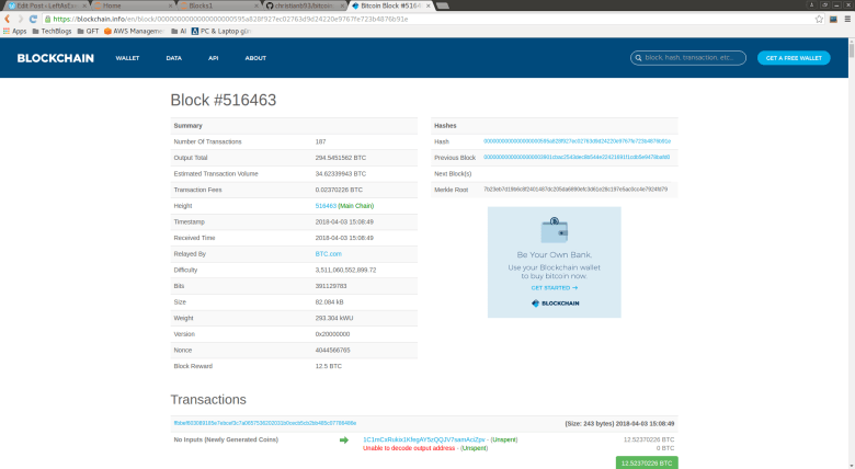
This output has a field bits that has the value 391129783. If you convert this into a hexadecimal string, you obtain 0x17502ab7, using for instance Pythons hex function. Now this function will give you the big-endian representation of the integer value. To convert to little endian as it can be found in the serialized format of a bitcoin block, you have to reverse the order byte wise and get b72a5017. If you now display the raw format of the block using this link and search for that string, you will actually find it at character 144 at expected.

Now on the screenshot above, you also see the difficulty displayed, which is a floating point number and is 3511060552899.72 in this case. How is that difficulty related to the bits?

As so often, we can find the answer in the bitcoin core source code, starting at the JSON RPC interface. So let us look at the function blockheaderToJSON in rpc/blockchain.cpp that is responsible for transforming a block in the internal representation into a human readable JSON format. Here we find the line

result.push_back(Pair("difficulty", GetDifficulty(blockindex)));

So let us visit the function GetDifficulty that we find in the same file, actually just a few lines up. Here we see that the bits are actually split into two parts. The first part, let me call this the size is just the value of the top 8 bits. The second part, the value of remaining 24 bits, is called the coefficient. Then the difficulty is calculated by dividing the constant 0xFFFF by the coefficient and shifting by 29 – size bits, i.e. according to the formula

$\text{difficulty} = 256^{(29 - \text{exponent})} \cdot (65535.0 / \text{coefficient})$

In Python, we can therefore use the following two lines to extract the difficulty from a block header in raw format.

nBits = int.from_bytes(bytes.fromhex(raw[144:152]), "little")
difficulty = 256**(29 - (nBits >> 24))*(65535.0 / ((float)(nBits & 0xFFFFFF)))

If you try this out for the transaction above, you will get 3511060552899.7197. Up to rounding after the second digit after the decimal point, this is exactly what we also see on the screenshot of blockchain.info. So far this is quite nice…

However, we are not yet done – this is not the only way to represent the difficulty. The second quantity we need to understand is the target. Recall that the mathematical puzzle that a miner needs to solve is to produce a block with a hash that does not exceed a given number. This number is the target. The lower the target, the smaller the range of 256 bit numbers that do not exceed the target, and the more difficult to solve that puzzle. So a low target implies high difficulty and vice versa.

In fact, there are two target values. One target is part of every block and stored in the bits field – we will see in a minute how this works. The second target is a global target that all nodes in the bitcoin network share – this value is updated independently by each node, but based on the same data (the blockchain) and the same rules so that they arrive at the same conclusion. A block considered valid if solves the mathematical puzzle according to the target which is stored in itself and if, in addition, this target matches the global target.

To understand how this works and the exact relation between target and difficulty, it is again useful to take a look at the source code. The relevant function is the function CheckProofOfWork in pow.cpp which is surprisingly short.

bool CheckProofOfWork(uint256 hash, unsigned int nBits, const Consensus::Params& params)
{
    bool fNegative;
    bool fOverflow;
    arith_uint256 bnTarget;

    bnTarget.SetCompact(nBits, &fNegative, &fOverflow);

    // Check range
    if (fNegative || bnTarget == 0 || fOverflow || bnTarget > UintToArith256(params.powLimit))
        return false;

    // Check proof of work matches claimed amount
    if (UintToArith256(hash) > bnTarget)
        return false;

    return true;
}

Let us try to understand what is going on here. First, a new 256 bit integer bnTarget is instantiated and populated from the bits (that are taken from the block) using the method SetCompact. In addition to a range check, it is then checked that the hash of the block does not exceed the target – this the mathematical puzzle that we need to solve.

The second check – verifying that the target in the block matches the global target – happens in validation.cpp in the function ContextualCheckBlockHeader. At this point, the function GetNextWorkRequired required is called which determines the correct value for the global target. Then this is compared to the bits field in the block and the validation fails if they do not match. So for a block to be accepted as valid, the miner needs to:

Actually solve the puzzle, i.e. provide a block with a hash value equal to or smaller than the current global target
Include this target as bits in the generated block

This leaves a couple of questions open. First, we still have to understand how the second step – encoding the target in the bits field – works. And then we have to understand how the global target is determined.

Let us start with the first question. We have seen that the target is determined from the bits using the SetCompact method of the class uint256. This function is in fact quite similar to GetDifficulty studied before. Ignoring overflows and signs for a moment, we find that the target is determined from the bits as

$\text{target} = \text{coefficient}\cdot 2^{8(\text{exponent}-3)}$

If we compare this to the formula for the difficulty that we have obtained earlier, we find that there a simple relation between them:

$\text{target} = \text{difficulty}^{-1}\cdot \text{std\_target}$

where std_target is the target corresponding to difficulty 1.0 and given by 0xFFFF shifted by 208 bits to the left, i.e. by 0xFFFF with 52 trailing zeros. So up to a constant, target and difficulty are simply inverse to each other.

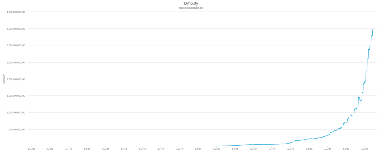
Now let us turn to the second question – how can the nodes agree on the correct global target? To see this, we need to look at the function GetNextWorkRequired. In most cases, this function will simply return the bits field of the current last block in the blockchain. However, every 2016 blocks, it will adjust the difficulty according to the following rule.

First, it will use the time stamps in the block to calculate how much time has passed since the block which is 2016 blocks back in the chain has been created – this value is called the actual time span. Then, this is compared with the target time span which is two weeks. The new target is then obtained by the formula (ignoring some range checks that are done to avoid too massive jumps)

$\text{target}_{new} = \text{target}_{old} \cdot \frac{\text{actual time span}}{\text{target time span}}$

Thus if the actual time span is smaller than the target time span, indicating that the mining power is too high and therefore the rate of block creation is too high, the target decreases and consequently the difficulty increases. This should make it more difficult for the miners to create new blocks and the block creation rate should go down again. Similarly, if the difficulty is too high, this mechanism will make sure that it is adjusted downwards. Thus the target rate is 2016 blocks being created in two weeks, i.e. 336 hours, which is a rate of six blocks per hours, i.e. 10 minutes for one block.

Finally, it is worth mentioning that there is lower limit for the difficulty, corresponding to a higher limit for the target. This limit is (as most of the other parameters that we have discussed) contained in chainparams.cpp and specific for the three networks main, net and regtest. For instance, for the main network, this is

consensus.powLimit = uint256S("00000000ffffffffffffffffffffffffffffffffffffffffffffffffffffffff");

whereas the same parameter for the regression testing network is

consensus.powLimit = uint256S("7fffffffffffffffffffffffffffffffffffffffffffffffffffffffffffffff");

This, together with the target of the genesis block (which determines the target for the first 2016 blocks) (bits = 0x207fffff ) determines the initial difficulty in a regression test network. Let us verify this (I knew I would somehow find a reason to add a notebook to this post…)

Sorry, something went wrong. Reload?

Sorry, we cannot display this file.

Sorry, this file is invalid so it cannot be displayed.

view raw InitialDifficultyRegTest.ipynb hosted with ❤ by GitHub

We are now well equipped to move towards our final project in this series – building a Python based miner. The last thing that we need to understand is how the miner operates and communicates with the bitcoin server, and this will be the topic of the next post.

Merkle trees

Suppose you are given a long file and wanted to use hashing to verify the integrity of the file. How would you do this in the most efficient way?

Of course, the first thing that might come to your mind is to simply take a hash of the entire file. This is very easy, but has one major disadvantage – if the file is damaged, there is no way to tell which part of the file has been damaged. If you use such a mechanism for instance to verify the integrity of a large download, you will have to go back and download the entire file again, which is very time consuming.

A smarter approach is to split the file into data blocks. You then calculate a hash for each data block to obtain a hash list. Finally, you could concatenate all the hashes into one large string and take the hash of that string. If a recipient of the file has access to only this top level hash, she could already verify the integrity of the file by repeating this procedure and comparing the top level hash with the hash created by the sender.

If that check fails, there is no need to re-transmit the entire file. Instead, the recipient could obtain a copy of the hash list itself and compare the hashes block by block until the faulty block is detected. This block can then be exchanged and the procedure can be repeated to verify that the replacement is valid. The bittorrent protocol uses this mechanism to detect inconsistencies in transferred files.

With a simple hash list like this, you would have to search the entire hash list in order to determine the faulty piece, requiring a time linear in the number of blocks. Searching can be improved greatly by organizing the hashes not into a list, but into a (binary) tree – and this data structure is called a hash tree or Merkle tree.

To illustrate the principle, suppose you wanted to build a hash tree for a file consisting of eight blocks, labeled 1 – 8.

You would then proceed as follows, as indicated in the image above. First, you compute the hash value for all blocks and assign them as values to the eight leaves of the tree. Then, you concatenate the values of leaves 1 and 2 and take the hash value of the result. This gives you the value for the parent node – called a in the picture above – of 1 and 2. You repeat the same procedure for the leaves 3 and 4, this gives you the value for the node b. Then you concatenate the values of a and b and take the hash value of the result, this gives you the value of the node c. Repeat this procedure for the right part of the tree and assign the result to node d. Finally, concatenate the values of node c and d and take the hash – this will be the value of the root node called the Merkle root. Thus, in a binary Merkle tree, the value of each node is defined to be the hash of the concatenation of the values of its two child nodes.

How is a Merkle tree realised in the bitcoin reference implementation? The currently relevant code is in consensus/merkle.cpp. This implementation is already optimized, the original implementation used to be in primitives/block.cpp and is still available on GitHub.

As the comments in the source code explain, at any level of the tree, the last node is added at the end again if needed to make sure that the number of nodes is even at each level – the algorithm that I have illustrated above only works if the number of leaves is a power of two. The actual implementation first builds a list of the leaves. It then goes through the list and for any two subsequent elements, it adds an element at the end which is the hash of the concatenation of these two elements. The last element is then the Merkle root that we are looking for.

Let us now see how a straightforward implementation looks like in Python.

Sorry, something went wrong. Reload?

Sorry, we cannot display this file.

Sorry, this file is invalid so it cannot be displayed.

view raw MerkleRoot.ipynb hosted with ❤ by GitHub

Most of the code should be self explaining, but a few remarks are in order. First, the hash function that we use could of course by any hash function, but, to be consistent with what bitcoin is doing, we use a double SHA256 hash. Then, byte ordering is again to be observed. The bitcoin reference client uses the method GetHash() on the involved transactions to populate the leaves, and we know that this is providing the transaction ID in little endian byte order. The entire calculation then proceeds in little endian byte order. The JSON output, however, display the transaction IDs in big endian order and the same holds for the Merkle root. Thus we need to reverse the byte order before we build the tree and, when comparing our result with the Merkle root which is part of the block, reverse the byte order again.

The actual calculation of the Merkle root uses a very straightforward approach – instead of maintaining one long list as the original bitcoin reference representation did, we represent the nodes at each level of the tree by a separate list and use recursion. This is probably a bit less efficient, but maybe easier to understand.

In order to test our implementation, we finally use the Python requests library to get a block in JSON format from blockchain.info using their REST API. We then build the leaves of the tree by walking through the list of transaction IDs in the block, build the Merkle root and compare the result to the value which is part of the JSON block structure. Nice to see that they match!

What happens if a client wants to verify that a given transaction is really included in a block without downloading the full block? In this case, it can ask the bitcoin server (either via the RPC call gettxoutproof or as part of the GETDATA network message) to provide a Merkle block, which is a serialized instance of CMerkleBlock. Essentially, a Merkle block consists of a block header plus a branch of the Merkle tree that is required to verify that a specific transaction is part of the block. This eliminates the need to transfer all transactions (which can be several thousand) while still allowing the client to check that a transaction is really included in a block.

This completes our short discussion of Merkle trees. We are now able to calculate the Merkle root for inclusion in a block header given the list of transactions that a block contains. To be able to mine a block, there is one more thing that we need to understand and that we will cover in the next post in this series – mining difficulty and the proof-of-work target.

Understanding bitcoin blocks

In order to analyse a block, obviously the first thing that we need is – a block. Fortunately, this is not difficult. We can either use the block explorer hosted by blockchain.info to get the second block in the blockchain in raw or JSON or use curl to retrieve the block from the command line, say in raw format.

$ curl https://blockchain.info/de/block/000000006a625f06636b8bb6ac7b960a8d03705d1ace08b1a19da3fdcc99ddbd?format=hex

010000004860eb18bf1b1620e37e9490fc8a427514416f
d75159ab86688e9a8300000000d5fdcc541e25de1c7a5a
ddedf24858b8bb665c9f36ef744ee42c316022c90f9bb0
bc6649ffff001d08d2bd61010100000001000000000000
0000000000000000000000000000000000000000000000
000000ffffffff0704ffff001d010bffffffff0100f205
2a010000004341047211a824f55b505228e4c3d5194c1f
cfaa15a456abdf37f9b9d97a4040afc073dee6c8906498
4f03385237d92167c13e236446b417ab79a0fcae412ae3
316b77ac00000000

For this post, I have chosen a block from the very early days of bitcoin, as this block contains only one transaction and is therefore rather small – current blocks typically contain more than 2.000 transactions and are too long to be displayed easily. This block is actually the third block on the blockchain and has height two. The height is the position of a block on the blockchain (ignoring forks). The block with height 0 is the very first block and actually hardcoded into the bitcoin software, this block is called the genesis block. The first blocks have all been mined (according to their time stamp) in the early morning hours of January 9th 2009.

If you want to follow this post step by step, I recommend to download and run the Jupyter notebook containing the respective code.

In order to understand a bitcoin block, let us again look at the source code of the reference implementation. If you have followed me through the dissection of a bitcoin transaction, you will not have any difficulties to understand the code in primitives/block.h and find that a block is made up of a block header (an instance of CBlockHeader) and the block data which is an instance of the derived class CBlock and contains, in addition to the header fields, the transactions that make up the block. Let us now go through the header fields one by one.

class CBlockHeader
{
public:
    // header
    int32_t nVersion;
    uint256 hashPrevBlock;
    uint256 hashMerkleRoot;
    uint32_t nTime;
    uint32_t nBits;
    uint32_t nNonce;

The first field is the version number, in the usual little endian encoding. Here, the version is simply 1 – not really surprising for the second block that was ever mined. In more recently mined blocks, the version field looks different and is most often 0x20000000 – this is not just a version number any more but a bit mask used to indicate any soft forks that the miner is willing to support, as specified in BIP 009.

The next field is the hash of the previous block. Similar to transactions, this in practice identifies a block uniquely (and is a better identifier than the position in the block chain since it also works for blocks in a fork). Actually, this is not really the hash of the entire block, but of the block header only (GetHash is a method of CBlockHeader).

If we compare the previous blocks hash ID with the JSON output, we find that compared to the JSON output, the order of the bytes is reversed. We have already seen that byte reversal when looking at transactions – the ID of the previous transaction also appears reversed in the serialization compared to the output of a blockchain explorer or the bitcoin-cli tool Time to look at why this happens in a bit more detail.

If you look at primitives/block.h, you will find that the hash of the previous transaction is a uint256. This data type – a 256 bit integer – is defined in uint256.h and is a number. As every number on the x86 platform (on which the bitcoin software was developed), this number is internally stored in little endian byte order, i.e. the least significant bit first (look for instance at the method base_blob::GetUint64 to see this) and is serialized as a little endian byte string (see base_blob::Serialize). However, if it is displayed, it is converted to a big endian representation in the the function base_blob::GetHex(), which simply reverts the order bytewise.

An example where this happens is the JSON RPC server. In blockheaderToJSON in rpc/blockchain.cpp, for instance, we find the line

if (blockindex->pprev)
        result.push_back(Pair("previousblockhash", blockindex->pprev->GetBlockHash().GetHex()));

So we see that GetHex() is called explicitly to convert the little endian internal representation of the hash into the big endian display format. This explains why the order of the hash appears to be reversed in the serialized raw format.

Having clarified this, let us now proceed with our analysis of the raw block data. The next field is called the Merkle root. Essentially, this is a hash value of the transactions which are part of the block, aggregated in a clever way, a so called Merkle tree. We will look at Merkle trees in a separate post, for the time being let us simply accept that this is a hash of the underlying transactions. Again, note that the order of the bytes is reversed between the JSON representation (big endian) and the serialized format (little endian).

The next field is again easy, it is the creation time of the block as announced by the miner who did build the block. As usual in the Unix world, the time is stored as POSIX time, i.e. essentially in seconds since the first of January 1970.

Again, byte order is significant – the hex string b0bc6649 in our case first needs to be reversed and then transformed into an integer:

nTime = nTime = int.from_bytes(bytes.fromhex('b0bc6649'), "little")
import time
print(time.ctime(nTime))

This should give you Friday, January 9th 2009 at 03:55:44.

The next field is called the bits – a name which would probably not win a prize for being a unique, meaningful and descriptive variable name. If you search the source code a bit, you will find that in fact, those bits represent the difficulty which controls the mining process – again, this is a matter for a separate post.

The last field in the header is again relevant for the mining process. It is called the nonce and is used as a placeholder that a miner can set to an arbitrary value in order to produce blocks with different hash values (actually, there is a second nonce hidden in the signature script of the coinbase transaction, we get to this point later when we discuss the mining in detail).

This completes the fields of the block header. In addition to these fields, a full block contains a vector holding the transactions that are contained in the block. As every vector, this vector is serialized by first writing out the number of elements – one in this case – followed by the individual transactions, encoded in the usual serialized format.

With this, we have completed our short tour through the layout of a block and are ready to summarize our findings in the following diagram.

In the next few posts, we will dig deeper into some of these fields and learn how Merkle trees are used to validate integrity and how the difficulty and the nonce play together in the mining process.

Quantum computing and the Blockchain

Browsing the MIT Technology Review, I recently found an article on the potential threat that quantum computing means for the bitcoin protocol in its current form. This article is in fact a review of a paper that appeared last October on the arxiv preprint server. If you use your favorite search engine and search for combinations of words like quantum computing, threat, bitcoin and cryptography, you find many articles on that topic with a greatly varying degree of accuracy – so it is definitely worth taking a look at that paper and see what it really says.

In the bitcoin protocol, computing power enters the picture at two vital points. The first point is the mining process. Recall that in order to create a new block, a mining node has to solve a mathematical challenge called the proof-of-work which is to adjust a part of the new block – the nonce – in such a way that the first few hexadecimal digits of the block hash become zero. The number of digits that need to be zero is controlled by the so called difficulty, a parameter of the network which is dynamically adjusted based on the mining rate, aimining at keeping the mining rate constant at roughly 6 blocks per hour.

So finding the nonce effectively amounts to inverting the used hash function (a double SHA256 hash). Currently, the only (at least publicly) known approach is brute force – simply try out a large number of values for the nonce in parallel and stop when you find a value that solves the puzzle.

On the site blockchain.info, you can find, among much additional information, a graphical history of the difficulty over time. At the time of writing, the development since the birth of the bitcoin looks as follows.

It appears that the difficulty has increased exponentially over the last years (the same web page also offers a version of that graph with a logarithmic scale which demonstrates that starting at 2015, the difficulty did in fact develop essentially exponentially over time). This can be used to estimate the number of hashes per second that are computed by all miners in the network together, and on blockchain.info, there is a nice graph illustrating the result. At the moment, the hash rate is estimated to be roughly 25.000 tera hashes per second, i.e. 2,5 * 10¹⁶ hashes per second, growing exponentially as well.

This dramatic increase in computing power devoted to mining is not just the result of more mining nodes participating in the network. It is also due to an evolution of the technology used to mine bitcoin. In 2010, miners started to use graphical processing units (GPUs), followed by FPGAs about one year later and finally by ASICS, i.e. custom manufactured integrated circuits which can only do one thing – computing hashes – but do this amazingly fast.

In [2], the authors investigate the question at which point in time quantum computing might be developed to the point where a quantum computer can solve the same challenge at a speed that is comparable to currently existing devices. Essentially, their conclusion is that it will easily take between 10 and fifteen years for this to pose a real threat for the bitcoin network. They estimate that quantum computers that can implement the required algorithms will not appear before 2018, and even then the speed of the quantum gates will be much lower than the speed of the custom built ASICS so that it will take in addition at least ten years until a single quantum computers reaches the range of hashing power that the entire bitcoin network represents. Thus, it is unlikely that we will soon see that a single quantum computer is able to run an attack against the bitcoin network based on hashing power.

However, there is a second threat that is much more realistic, targeting the second point in the bitcoin protocol where computing power is essential – the signature algorithm based on elliptic curve cryptography.

In fact, elliptic curve cryptography is based on the difficulty to calculate a discrete logarithm on a classical computer, and was one of the first problems for which it could be shown (see [3]) that it could be solved using a quantum computer much faster, i.e. polynomial in the number of inputs.

In [2], a few attack scenarios are described and one specific scenario is analysed in detail. To understand this scenario, suppose that Alice is creating a transaction to transfer bitcoin to Bob. When she uses the standard P2PKH signature scheme, that transaction will contain the hash value of Bobs public key, but the full public key of Alice. So when this transaction appears on the network, the public key is known. If an attacker is able to solve the discrete logarithm that is required to derive the private key from the public key (see this post for the relation between public and private key), the attacker can use the private key to create an own transaction to spend the UTXO that Alice is using. That attack would have to be executed before the original transaction is added to a block, thus within less than 10 minutes.

The authors then determine how many qubits a quantum computer would need to solve the discrete logarithm and again predict, based on the current rate of improvement of quantum computing technology, how long it would take until a first quantum computer becomes available that can solve this in less than 10 minutes. Different scenarios are considered, but in the most aggressive scenario, this will happen in 2027, i.e. less than ten years from now.

So the conclusion is that the most serious threat to the bitcoin protocol in its current form comes from the anticipated ability of quantum computers to quickly break the ECDSA algorithm in less than ten years from now. Fortunately, the authors also propose countermeasures. In fact, there are public key signature algorithms that appear to be quantum safe, i.e. for which no quantum algorithm is known which can solve the underlying mathematical challenge faster than on traditional hardware. So it is possible to adapt the bitcoin protocol in a way that makes it less vulnerable to attacks by quantum computers.

Thus the key take aways from the paper seem to be that quantum computing will most likely not kill the bitcoin protocol, but force it to change – and that we still have a few years to go even under optimistic assumptions on the rate of further improvement of quantum computing technology.

References

1. L. Cocco, M. Marchesi, Modeling and Simulation of the Economics of Mining in the Bitcoin Market, PLoS One 11 (10) (2016)
2. D. Aggarwal et al., Quantum attacks on Bitcoin, and how to protect against them
3. P. W. Shor. Polynomial-Time Algorithms for Prime Factorization and Discrete Logarithms on a Quantum Computer. SIAM Review, 41(2):303–332, 1999 (see also the preprint on the arxiv)

Bitcoin mining – an overview

In my recent posts in this series, I have walked you in detail through two of the basic objects that make up the bitcoin blockchain – participants, represented by public / private key pairs, and transactions. Time to look at the third major ingredient – blocks.

What are blocks and why are they necessary? When the bitcoin protocol was invented in 2008 by a person (or group of persons) acting under the pseudonym Satoshi Nakamoto (see [1]), the real novelty was not the usage of a chain of transactions in order to model payments. The real novelty was the proposed solution for a major issue with a cryptocurrency that is based solely on such a chain: the problem of double spending. To understand this, suppose that Eve agrees on a deal with Alice: Eve will transfer a certain amount of bitcoin to Alice in exchange for another currency like USD. She would pick an unspent transaction output of the correct amount, create and sign a transaction and publish that transaction in the network. Alice could see and validate the transaction appearing in the network and would then transfer the USD amount to Eve.

Unfortunately, Eve could, at virtually the same time, agree on a similar deal with Bob and create another transaction transferring the same unspent output to Bob.

Now we have two transactions in the network that both claim to spend the same previously unspent transaction output. However, what if, due to some network latency, Bob and Alice detect the second transaction only after they have initiated the transfer of the USD amount? And if they detect the problem, how can they – and the entire network – agree on which of these transactions should be considered valid and which should be discarded? This is the double spend problem.

To solve this, a mechanism is needed that allows all nodes of the network to agree on an order of transactions. If we have that order, the solution to our problem is easy – the first transaction, i.e. the transaction with the lowest order wins. Satoshis proposal was to implement an ordering by what he called a timestamp service and what is now known as the blocks of the blockchain.

Essentially, blocks are groups of transactions. Nodes in a bitcoin network collect transactions that have been posted, but not yet included in a block. They then calculate hash values of these transactions and organize them into a larger data structure – the block. But similar to transactions, blocks are linked into a chain – Satoshi calls this proof-of-work chain and in fact the term blockchain does not appear at all in his paper but was introduced later. Each (full) node in the network maintains a local copy of this chain. Whenever a node creates a block, it includes the hash value of the current last block in the chain in the block data structure. It then publishes the block on the network. If other nodes pick up the block, they can verify that it is valid – in particular they can verify that none of the transactions included in the block lead to double spending with respect to any other transaction in this or earlier blocks. If this validation is successful, the block is added to the copy of the chain maintained by the server.

The fact that the blocks in the chain are linked makes it more difficult to alter a block (and the transactions contained in it) that is already buried below some new blocks. In fact, in order to do this, we would have to recreate all blocks between the current last block and the block that we want to alter, as the blocks contain hash values of their predecessor. In order to make sure that this is virtually undoable, every node that creates a block needs to solve a mathematical puzzle – a so called proof of work. The difficulty of this puzzle can be adjusted dynamically and is kept at a level where approximately 10 minutes of work are required to create a new block. This also makes it less likely that new blocks are created at exactly the same point in time.

In the bitcoin block chain, this proof of work is designed as follows. The block data structure contains hash values of the transactions that are part of the block and – in addition – a field called the nonce that the node creating the block can determine at will. As the nonce enters the hash value of the block, this implies that, simply by trying out different values for the nonce, a node can create blocks whose hash value has certain properties. The mathematical challenge that a node has to solve to create a block that is accepted by the network is to adjust the nonce such that the hash value of the block is zero in the first few hexadecimal digits. The number of leading digits that need to be zero is the difficulty which is adjusted over time to make sure that the block creation rate is kept at one block per ten minutes.

Thus a node that wishes to create a new block will collect transactions not yet included in a block, verify them (and will thereby avoid double spend), add them to a block along with the hash of the current last block, try out some value of the nonce, calculate the hash value, check whether its first digits are zero, try a different nonce if that is not the case and so on until a matching nonce is found. Then the block is published, verified by the other nodes and – if it passes the checks – added to the block chain as the next block. Nodes that create new blocks are called miners.

Let us now trace the full history of a sample transaction throughout this process.

Suppose Alice wants to transfer 50 BTC to Bob. She creates and signs a transaction according to the rules that we have seen in the previous posts. That transaction is then published in the network. A mining node picks up the transaction and assembles it – along with many other transactions – in a new block. That block is then distributed on the network. Each node on the network validates the block and adds it to the copy of the blockchain that this node maintains. Finally, Bob can listen on the network as well. As soon as Bob finds that the transaction has been added to a block and this block has been included in the network, he can be relatively sure that the transaction is valid. Bob can now be confident to be protected against double spend and use this transaction in turn as unspent output (as a rule of thumb, a transaction is considered to be confirmed if it is included in a block and at least five additional blocks have been added on top of that, i.e. after roughly one hour).

There are still a few open ends. Why, for instance, should a mining node invest CPU power in the creation of blocks? And what happens if two different blocks are mined at the same time?

Let us first start with the question of incentivation. In order to make sure that miners participate in the process, a miner is rewarded for every block that he creates. In fact, each new block contains a special transaction called a coinbase transaction. Such a transaction has no inputs, and the mining node can determine the address to which the output is credited. Thus, effectively, mining creates bitcoins, and the miner earns the newly created bitcoins.

The amount of a coinbase transaction used to be 50 BTC in the first days of the bitcoin protocol, and is halved every 210.000 blocks. At the moment, the reward is 12.5 BTC, which is the equivalent of roughly 10.000 USD at the current exchange rate. This is the incentive for the mining node to invest energy and hardware cost into the process.

Now let us see what happens if two valid blocks are mined at the same time. In this case, we create a fork of the chain.

Suppose, for instance, that two different nodes find a solution for the mathematical puzzle at exactly the same point in time and publish two blocks that could fit into position N of the chain. Let us call these blocks N and N’. Now all the other nodes in the network have to take a decision which chain they consider to be the main chain – the chain continued with N or the chain continued with N’. There is one basic rule in this game – the longest chain wins. However, at this point in time, both chains have the same length. So some of the nodes – say roughly half of them – will opt for the first chain, the other part of the nodes will opt for the second chain. Now each mining node will continue to work on the chain that this node considers to be valid. So roughly 50% of the miners will start to work on a block which could follow block N and the other nodes will start to search for a block that could follow N’.

Now it is rather unlikely that again, both puzzles are solved at exactly the same point in time. So let us assume that the next block which is mined is based on N. This block will then be published. Now the chain based on N is longer than the chain based on N’, and all the other nodes will – according the rule that the longest chain is the winning chain – discard the chain based on N’ and continue to mine blocks based on the new chain that included N. Thus the fork is resolved and all chains agree again on one copy of the chain.

That completes our short overview of the mining process. In the next couple of posts, we will again analyze the structure of a block in detail and see whether we will eventually be able to mine and publish a block in our test network.

References

1. Satoshi Nakamoto, Bitcoin: A Peer-to-Peer Electronic Cash System, 2008
2. Bitcoin History: Pre-Blockchain Digital Currencies

Creating and signing a bitcoin transaction from scratch

In the one of the the last posts in this series, we have been able to successfully verify an existing bitcoin transaction. With the understanding of how this works, we should now be able to conversely create a transaction from scratch, sign it and publish it in the bitcoin network.

Given an amount that we want to transfer and the target, we will first need to determine unspent transaction outputs which are available and select those UTXOs that we will be using. This process is called coin selection. Coin selection is a non-trivial task, as it needs to consider several variables like the number of coins in your wallet, the size of the resulting transaction, and the required fee to make sure that the transaction is picked up and included in a block by a miner. In the bitcoin reference implementation, coin selection is done in the method CWallet::SelectCoins in the file wallet.cpp. The logic is nicely described in this post on StackExchange. Essentially, it will first try to spend all those outputs that are smaller than the target amount. If that does not give an exact match, it will try to find a single output larger than the target amount. Otherwise, it will select a random subset of those outputs smaller than the target. Other algorithms exists, and I even found a masters thesis on this on the web (see [2]).

For our purpose, we will implement an easier algorithm that I have seen in the excellent book [1]. Again, we will be using the btc package that is available in my GitHub repository. The first thing that we do is to retrieve a list of all unspent transaction outputs that our wallet knows. To do this, we again use the RPC interface to access the wallet built into the bitcoin core client and call the method listunspent. We then split the resulting list of coins in two lists – one containing all entries smaller than the amount to spend, the other one containing all other entries.

#
# First we make an RPC call to retrieve unspent transaction output and 
# select the outputs that we are going to spend
#
listunspent = btc.utils.rpcCall("listunspent")
#
# Now extract transaction IDs and store that in a list of 
# dictionaries
#
# We split this list into one list of entries that are greater
# than the amount we want to transfer and one list of entries
# that are smaller
#
#
smaller = []
greater = []
amount_to_spend = float(args.amount)
for _ in listunspent:
    if _['spendable']:
        txid = _['txid']
        vout = _['vout']
        amount = float(_['amount'])
        address = _['address']
        coin = {'txid': txid,
                  'vout': vout,
                  'amount': amount,
                  'address' : address}
        if amount > amount_to_spend:
            greater.append(coin)
        else:
            smaller.append(coin)

Next we sort these two lists and build a list to_be_spent of those coins that we want to spend. If there is a coin that is greater than the amount to be spend, we take this entry and are done. If not, we try to sum up available coins from the other list to reach our target sum.

#
# Next we sort the lists. 
#
greater.sort(key=lambda entry: entry['amount'])
smaller.sort(key=lambda entry: entry['amount'], reverse=True)
#
# If greater is not emtpy, take the smallest (i.e. now first)
# element
#
if len(greater) > 0:
    amount_funded = greater[0]['amount']
    to_be_spent = [greater[0]]
else:
    #
    # We need to combine more than one transaction output
    #
    to_be_spent = []
    amount_funded = 0
    for _ in smaller:
        if amount_funded < amount_to_spend:
            to_be_spent.append(_)
            amount_funded += _['amount']
    if (amount_funded < amount_to_spend):
        # Failed, clean up list
        to_be_spent = []

Now that we have selected the UTXOs that we will use to build our transaction, we need to retrieve the corresponding private keys so that we can use them for the needed signatures. At the same time, we will build a list of the transaction outputs that we use in our standard format (i.e. as Python objects).

txos = []
privateKeys = []
for _ in to_be_spent:
    tx = btc.txn.txn()
    raw = btc.utils.rpcCall("getrawtransaction", [_['txid']])
    tx.deserialize(raw)
    #
    # Get private key using again an RPC call 
    #
    privKey = btc.utils.rpcCall("dumpprivkey", [_['address']])
    privKey = btc.keys.wifToPayloadBytes(privKey)
    privKey = int.from_bytes(privKey, "big")
    privateKeys.append(privKey)
    txos.append(tx.getOutputs()[_['vout']])

We can now assemble our transaction. We will only use one transaction output for simplicity. WARNING: this will imply that the difference between the amount represented by our unspent transaction outputs and the amount that we want to transfer counts as fees and will be lost! In our example, we use an UTXO worth 30 bitcoin and transfer only one bitcoin, i.e. we will loose almost 29 bitcoin which is almost 30 kUSD at the current bitcoin / USD exchange rate! So do not do this with real bitcoin.

Here is the code to assemble our transaction.

#
# Next we create our transaction. First we create the transaction 
# inputs. We leave the signature scripts empty for the time
# being
#
txn = btc.txn.txn()
for _ in to_be_spent:
    txin = btc.txn.txin(prevTxid = _['txid'], vout = _['vout'])
    txn.addInput(txin)

#
# Next we do the outputs. For the time being, we use only one output
# So we need to convert the address to a public key hash
#
publicKeyHash = btc.keys.ecAddressToPKH(args.target)
publicKeyHash = binascii.hexlify(publicKeyHash).decode('ascii')
#
# Create locking script
#
lockingScript = btc.script.scriptPubKey(scriptType = btc.script.SCRIPTTYPE_P2PKH, 
                                        pubKeyHash = publicKeyHash)
#
# and output
#
txout = btc.txn.txout(value = int(amount_to_spend * 100000000), 
                      scriptPubKey = lockingScript)
txn.addOutput(txout)

Next we need to sign our transaction, i.e. we need to go through all transaction inputs and add the correct signatures. We already know how to do this – simply revert the process that we have studied in my previous post. I have put the required code into the function signTransaction in the module btc.script. The only subtlety that we have to observe is that the ECDSA signature algorithm might return a pair (r,s) where s is greater than n/2 – such a signature would be rejected by the bitcoin client (see the check in interpreter.cpp/IsLowDERSignature). Therefore we need to replace s by n – s if needed. With this function, signing and sending is now very easy.

#
# Sign it
#
txn = btc.script.signTransaction(txn, txos, privateKeys)
#
# and send it
#
raw = txn.serialize()
s = btc.utils.rpcCall("sendrawtransaction", [raw, True])
print("Done, resulting transaction ID: ")
print(s)

Now let us actually run this and try it out. To be a bit more realistic, we will first create a third node called Bob in our test network. Using our stored containers, this is very easy. We can use the following command to bring up a container called Bob and – in addition – an instance of our previously created Alice container.

$ docker run -d --rm -p 18332:18332 --name=alice alice
$ docker run -it --rm --name=bob bitcoin-alpine

Now let us add a new address to Bob’s wallet that we will use as target address for our transaction. We can use the bitcoin-cli client if we first attach to the container bob

$ docker exec -it bob sh
# bitcoin-cli --rpcuser=user --rpcpassword=password -regtest getnewaddress "Bob"
n37U5uEL2h9FcZbumpoAxNYT9ACGjZCkCi

The output is the new address that we have just generated. If you now run the listaccounts command in the same terminal, you will see the newly created account and its balance which is still zero.

Now switch back to a terminal on your host. Clone my repository and run the script SendMoney.

$ git clone http://www.github.com/christianb93/bitcoin.git
$ cd bitcoin
$ python SendMoney.py --target=n37U5uEL2h9FcZbumpoAxNYT9ACGjZCkCi

Note that the argument --target is the newly created address. We are now almost done, but two steps remain. First, we will again have to connect our two nodes. As in the previous post, run docker network inspect bridge to find out the IP address of the node alice on the bridge network. In my case, this is again 172.17.0.2. Then reattach the terminal to the container bob and connect to this peer.

$ docker exec -it bob sh
# bitcoin-cli --rpcuser=user --rpcpassword=password -regtest addnode "172.17.0.2" add

Finally, we need to include our newly created transaction in the blockchain, i.e. we have to go through the process of mining again. For the sake of simplicity, we will use the container of Alice as its port 18332 is mapped into the host network and so we can reach it from our host and use the bitcoin CLI client there. So on the host (!) open a terminal and run

$ bitcoin-cli --rpcuser=user --rpcpassword=password -regtest generate 6

As a result, you should see the IDs of the six newly created blocks. Now let us switch back to the terminal attached to Bob and check the balance.

# bitcoin-cli --rpcuser=user --rpcpassword=password -regtest listaccounts
{
  "": 0.00000000,
  "Bob": 1.00000000
}

Aaaahh, the sweet taste of success – we made it. Our transaction has been accepted by the network, enclosed into a block and correctly interpreted by Bobs node as contributing one bitcoin to his balance.

This post completes our in-depth analysis of transactions in the bitcoin blockchain. With the next post, we will switch our focus and start to investigate the process of mining and the structure of blocks in detail.

1. A. Antonopoulos, Mastering Bitcoin, O’Reilly 2015
2. M. Erhardt, An evaluation of coin selection strategies, Masters Thesis, Karlsruhe Institute of Technology, available at this URL

Setting up and testing our bitcoin network

In the last post in my series on bitcoin and the blockchain, we have successfully “dockerized” the bitcoin core reference implementation and have built the bitcoin-alpine docker container that contains a bitcoin server node on top of the Alpine Linux distribution. In this post, we will use this container image to build up and initialize a small network with three nodes.

First, we start a node that will represent the user Alice and manage her wallet.

$ docker run -it --name="alice" -h="alice" bitcoin-alpine

Note that we have started the container with the option -it so that it stays attached to the current terminal and we can see its output. Let us call this terminal terminal 1. We can now open a second terminal and attach to the running server and use the bitcoin CLI to verify that our server is running properly.

$ docker exec -it alice  "sh"
# bitcoin-cli -regtest --rpcuser=user --rpcpassword=password getinfo

If you run – as shown above – the bitcoin CLI inside the container using the getbalance RPC call, you will find that at this point, the balance is still zero. This not surprising, our network does not contain any bitcoins yet. To create bitcoins, we will now bring up a miner node and mine a certain amount of bitcoin. So in a third terminal, enter

$ docker run -it --name="miner" -h="miner" bitcoin-alpine

This will create a second node called miner and start a second instance of the bitcoin server within this network. Now, however, our two nodes are not yet connected. To change this, we can use the addnode command in the bitcoin CLI. So let us figure out how they can reach each other on the network. We have started both containers without any explicit networking options, so they will be connected to the default bridge network that Docker creates on your host. To figure out the IP addresses, run

$ docker network inspect bridge

on your host. This should produce a list of network devices in JSON format and spit out the IP addresses of the two nodes. In my case, the node alice has the IP address 172.17.0.2 and the miner has the IP address 172.17.0.3. So let us change back to terminal number 2 (attached to the container alice) and run

# bitcoin-cli -regtest --rpcuser=user --rpcpassword=password addnode 172.17.0.3 add

In the two terminal windows that are displaying the output of the two bitcoin daemons on the nodes alice and miner, you should now see an output similar to the following.

2018-03-24 14:45:38 receive version message: /Satoshi:0.15.0/: version 70015, blocks=0, us=[::]:0, peer=0

This tells you that the two peers have exchanged a version message and recognized each other. Now let us mine a few bitcoins. First attach a terminal to the miner node – this will be terminal four.

$ docker exec -it miner "sh"

In that shell, enter the following command

# bitcoin-cli -regtest --rpcuser=user --rpcpassword=password generate 101
# bitcoin-cli -regtest --rpcuser=user --rpcpassword=password getbalance

You should now see a balance of 50 bitcoins. So we have mined 50 bitcoins (in fact, we have mined much more, but it requires additional 100 blocks before a mined transaction is considered to be part of the balance and therefore only the amount of 50 bitcoins corresponding to the very first block shows up).

This is already nice, but when you execute the RPC method getbalance in terminal two, you will still find that Alice balance is zero – which is not surprising, after all the bitcoins created so far have been credited to the miner, not to Alice. To change this, we will now transfer 30 bitcoin to Alice. As a first step, we need to figure out what Alice address is. Each wallet maintains a default account, but we can add as many accounts as we like. So let us now add an account called “Alice” on the alice node. Execute the following command in terminal two which is attached to the container alice.

# bitcoin-cli -regtest --rpcuser=user --rpcpassword=password getnewaddress "Alice"

The output should be something like mkvAYmgqrEFEsJ9zGBi9Z87gP5rGNAu2mx which is the bitcoin address that the wallet has created. Of course you will get a different address, as the private key behind that address will be chosen randomly by the wallet. Now switch to the terminal attached to the miner node (terminal four). We will now transfer 30 bitcoin from this node to the newly created address of Alice.

# bitcoin-cli -regtest --rpcuser=user --rpcpassword=password sendtoaddress "mkvAYmgqrEFEsJ9zGBi9Z87gP5rGNAu2mx" 30.0

The output will be the transaction ID of the newly created transaction, in my case this was

2bade389ac5b3feabcdd898b8e437c1d464987b6ac1170a06fcb24ecb24986a8

If you now display the balances on both nodes again, you will see that the balance in the default account on the miner node has dropped to something a bit below 20 (not exactly 20, because the wallet has added a fee to the transaction). The balance of Alice, however, is still zero. The reason is that the transaction does not yet count as confirmed. To confirm it, we need to mine six additional blocks. So let us switch to the miners terminal once more and enter

# bitcoin-cli -regtest --rpcuser=user --rpcpassword=password generate 6

If you now display the balance on the node alice, you should find that the balance is now 30.

Congratulations – our setup is complete, we have run our first transaction and now have plenty of bitcoin in a known address that we can use. To preserve this wonderful state of the world, we will now create two new images that contain snapshots of the nodes so that we have a clearly defined state to which we can always return when we run some tests and mess up our test data. So switch back to a terminal on your host and enter the following four commands.

$ docker stop miner
$ docker stop alice
$ docker commit miner miner
$ docker commit alice alice

If you now list the available images using docker images, you should see two new images alice and miner. If you want, you can now remove the stopped container instances using docker rm.

Now let us see how we can talk to a running server in Python. For that purpose, let us start a detached container using our brand new alice image.

$ docker run  -d --rm --name=alice -p 18332:18332 alice

We can now communicate with the server using RPC requests. The bitcoin RPC interface follows the JSON RPC standard. Using the powerful Python package requests, it is not difficult to write a short function that submits a request and interprets the result.

def rpcCall(method, params = None, port=18332, host="localhost", user="user", password="password"):
    #
    # Create request header
    #
    headers = {'content-type': 'application/json'}
    #
    # Build URL from host and port information
    #
    url = "http://" + host + ":" + str(port)
    #
    # Assemble payload as a Python dictionary
    # 
    payload = {"method": method, "params": params, "jsonrpc": "2.0", "id": 1}        
    #
    # Create and send POST request
    #
    r = requests.post(url, json=payload, headers=headers, auth=(user, password))
    #
    # and interpret result
    #
    json = r.json()
    if 'result' in json and json['result'] != None:
        return json['result']
    elif 'error' in json:
        raise ConnectionError("Request failed with RPC error", json['error'])
    else:
        raise ConnectionError("Request failed with HTTP status code ", r.status_code)

If have added this function to my btc bitcoin library within the module utils. We can use this function in a Python program or an interactive ipython session similar to the bitcoin CLI client. The following ipython session demonstrates a few calls, assuming that you have cloned the repository.

In [1]: import btc.utils
In [2]: r = btc.utils.rpcCall("listaccounts")
In [3]: r
Out[3]: {'': 0.0, 'Alice': 30.0}
In [4]: r = btc.utils.rpcCall("dumpprivkey", ["mkvAYmgqrEFEsJ9zGBi9Z87gP5rGNAu2mx"])
In [5]: r
Out[5]: 'cQowgjRpUocje98dhJrondLbHNmgJgAFKdUJjCTtd3VeMfWeaHh7'

We are now able to start our test network at any time from the saved docker images and communicate with it using RPC calls in Python. In the next post, we will see how a transaction is created, signed and propagated into the test network.

Building a bitcoin container with Docker

When we are playing with bitcoin transactions, we need some playground where making a mistake does not cost us real bitcoins and therefore money. In addition, we might want to play around with more than one bitcoin server to see how networkings works and how the messages are exchanged in the bitcoin peer-to-peer network.

There are several ways to do this. First, we could run more than one bitcoin server locally, and use different data directories and different configuration files and ports to separate them. However, there is a different option – we can use Docker container. This will make it ease to spin up as many instances as needed while only having to put together the configuration once, supports networking and allows us to easily clean up after we have tried something and restart our scenarios from a well defined state. In this post, I will guide you through the steps needed to build and install the bitcoin core software inside a container. This post is not meant to be a general introduction into container technology and Docker, but do not worry – I will not assume that you are familiar with the concepts, but we will start from scratch. However, if you want to understands the basics, there are many good posts out there, like this introduction or the Docker overview page which is part of the official documentation.

First, we will need to make sure that we have the latest Docker CE installed. On Ubuntu 16.04, this requires the following steps. First, we need to remove any potentially existing docker versions.

$ sudo apt-get remove docker docker-engine docker.io

Next we will add the Docker repository to the repository list maintained by APT to be able to install from there. So we first use curl to get the public key from the docker page, feed this into the apt-key tool and then add the repository.

$ curl -fsSL https://download.docker.com/linux/ubuntu/gpg | sudo apt-key add - 
$ sudo add-apt-repository "deb [arch=amd64] https://download.docker.com/linux/ubuntu xenial stable"

We can then install docker from there and make sure that it is started at boot time using

$ sudo apt-get update
$ sudo apt-get install docker-ce
$ sudo systemctl enable docker

You also should make sure that there is a docker group to which your user is added – use the command groups to verify that this is the case and follow the instructions on the Docker page if not.

When everything is done, let us test our installation. We will ask docker to download and run the hello-world minimal image.

$ docker run hello-world Unable to find image 'hello-world:latest' locally latest: Pulling from library/hello-world ca4f61b1923c: Pull complete Digest: sha256:97ce6fa4b6cdc0790cda65fe7290b74cfebd9fa0c9b8c38e979330d547d22ce1 Status: Downloaded newer image for hello-world:latest


Hello from Docker!

This message shows that your installation appears to be working correctly.
To generate this message, Docker took the following steps:

 1. The Docker client contacted the Docker daemon.

 2. The Docker daemon pulled the "hello-world" image from the Docker Hub.

    (amd64)

 3. The Docker daemon created a new container from that image which runs the

    executable that produces the output you are currently reading.

 4. The Docker daemon streamed that output to the Docker client, which sent it

    to your terminal.
To try something more ambitious, you can run an Ubuntu container with:

 $ docker run -it ubuntu bash
Share images, automate workflows, and more with a free Docker ID:

 https://cloud.docker.com/

For more examples and ideas, visit: https://docs.docker.com/engine/userguide/

Now we can start with the actual installation. At the end, of course, there will be a Dockerfile – but I will guide you through the individual steps one by one and we will create the final file iteratively. If you would only like to see the result, you can skip to the last paragraph of this post that explains how to retrieve this file from my GitHub repository and to use it … but if course you are more than welcome to join me on the way there.

Actually, we will even do a bit more than we would need if we only wanted to have a running bitcoind, but this post is also meant as a refresher if you have built docker images before and as a hands-on introduction if you have never done this.

As a basis, we will use the Alpine Linux distribution. From there, we have several options to proceed. Of course, the Alpine Linux distribution has a docker package, but simply that or any other precompiled binary would not give us the flexibility that we need – it is for instance extremely useful to be able to add debugging output to the source code if something is not as expected. Besides, it is more fun to compile from scratch. So our target will be to pull the source code, compile and install in a container.

Based on the Alpine Linux container, we will first create several container images with separate docker files that are based on each other, which will make it easier to iterate and check things manually as we go. In the end, we will assemble everything into one docker file.

As a first step, we add a few libraries to the Alpine image that we need to be able to fetch and compile the bitcoin source code. We call the target image alpine-dev as it can be reused as a development environment for other purposes as well. Here is the docker file Dockerfile.dev

FROM alpine
RUN apk update && apk add git \ 
                          make \
                          file \
                          autoconf \
                          automake \ 
                          build-base \
                          libtool \
                          db-c++ \
                          db-dev \
                          boost-system \
                          boost-program_options \
                          boost-filesystem \ 
                          boost-dev \ 
                          libressl-dev \ 
                          libevent-dev

Save this file somewhere in a local directory (ideally, this directory is otherwise empty as during the build process, its context will be transferred to the docker daemon and used as build context, so we better keep this small) and then build the image using

docker build -f Dockerfile.dev -t alpine-dev .

If you now check your local repository with docker images, you should see that the image has been added successfully (it is big, but do not worry, we fix that later).

The next image that we will be building is an image that is based on alpine-dev but contains the specific version of the bitcoin source code that we want, i.e. it pulls the code from the bitcoin directory. So its docker file is very short.

FROM alpine-dev
RUN git clone https://github.com/bitcoin/bitcoin --branch v0.15.0 --single-branch

You can build this image with

docker build -f Dockerfile.build -t bitcoin-alpine-build .

Next we write the docker file that performs the actual build. This is again not difficult (but here it comes in handy that we can run a container from the image that we have just generated and play around with the configuration to arrive at the final set of options below).

FROM bitcoin-alpine-build
RUN (cd bitcoin  && ./autogen.sh && \
                      ./configure --disable-tests \
                      --disable-bench --disable-static  \
                      --without-gui --disable-zmq \ 
                      --with-incompatible-bdb \
                      CFLAGS='-w' CXXFLAGS='-w' && \
                      make -j 4 && \
                      strip src/bitcoind && \
                      strip src/bitcoin-cli && \
                      strip src/bitcoin-tx && \
                      make install )

Again, we build the image and place it into our local repository using

docker build -f Dockerfile.install -t bitcoin-alpine-bin .

Let us now test our installation. We first bring up an instance of our new container.

docker run -it bitcoin-alpine-bin

Within the container, we can now run the bitcoin daemon.

bitcoind -server=1 -rest=1 -regtest -txindex=1 -daemon

Once the daemon has started, we can verify that it is up and running and ready to accept commands. We can for instance – from within the container – run bitcoin-cli -regtest getinfo and should see some status information.

So let us now move on to write the docker file that will create the run time environment for our daemon. There is still a couple of things we need to think about. First, we will have to communicate with our bitcoin server using JSON-RPC, so we need to expose this port towards the host.

Second, we need a configuration file. We could generate this on the fly, but the easiest approach is to place this in the build context and copy it when we run the daemon.

Finally, we have to think about the RPC authorization mechanism. Typically, the bitcoin server writes a cookie file into the configuration directory which is then picked up the by client, but this does not work if the server is running inside the container and the client locally on our host system. Probably the safest way would be to use the option to provide a hashed password to the server and keep the actual password secure. We will use a different approach which is of course not recommended for production use as it could allow the world access to your wallet – we specify the username and password in the configuration file. Our full configuration file is

regtest=1
server=1
rpcbind=0.0.0.0:18332
rpcuser=user
rpcpassword=password
rpcallowip=0.0.0.0/0
rpcport=18332
rpcuser=user
rpcpassword=password

Note that this opens the RPC port to the world and is probably not secure, but for use in a test setup this will do. Our docker file for the last stage is now

FROM bitcoin-alpine-bin

#
# Copy the bitcoin.conf file from
# the build context into the container
#
COPY bitcoin.conf /bitcoin.conf

#
# Expose the port for the RPC interface
#
EXPOSE 18332/tcp

#
# Start the bitcoin server
#
ENTRYPOINT ["/usr/local/bin/bitcoind"]
CMD ["-conf=/bitcoin.conf", "-regtest", "-rest=1", "-server=1", "-printtoconsole", "-txindex=1"]

We can now test our client. First, we build and run the container.

$ docker build -f Dockerfile.run -t bitcoin-alpine-run . $ docker run --rm -it -p 18332:18332 bitcoin-alpine-run

Then, in a second terminal, let us connect. We assume that you have an installation of the bitcoin-cli client on the host machine as well. Run

$ bitcoin-cli -regtest -rpcuser=user -rpcpassword=password getinfo

You should now see the usual output of the getinfo command similar to the test that we have done before directly in the container.

That is nice, but there is a serious issue. If you look at the image that we have just created using docker images, you will most likely be shocked – our container is more than 800 Mb in size. This is a problem. The reason is that our image contains everything that we have left behind during the build process – the development environment, header files, the source code, object files and so on. It would be much nicer if we could build a clean image that only contains the executables and libraries needed at runtime.

Fortunately, current versions of Docker offer a feature called multi-stage build which is exactly what we need. Let us take a look at the following docker file to explain this.

FROM bitcoin-alpine-bin as build

RUN echo "In build stage"

FROM alpine

#
# Copy the binaries from the build to our new container
#
COPY --from=build /usr/local/bin/bitcoind /usr/local/bin

#
# Install all dependencies
#
RUN apk update && apk add boost boost-filesystem \
            boost-program_options \
            boost-system boost-thread busybox db-c++ \
            libevent libgcc libressl2.6-libcrypto \ 
            libstdc++ musl

#
# Copy the bitcoin.conf file from
# the build context into the container
#
COPY bitcoin.conf /bitcoin.conf

#
# Expose the port for the RPC interface
#
EXPOSE 18332/tcp

#
# Start the bitcoin server
#
ENTRYPOINT ["/usr/local/bin/bitcoind"]
CMD ["-conf=/bitcoin.conf", "-regtest", "-rest=1", "-server=1", "-printtoconsole", "-txindex=1"]

We see that this docker file has two FROM statements. When it is executed, it starts with the image specified by the first FROM statement. In our case, this is the bin image that did already contain the executable binaries. In this stage, we do nothing in our simple example but simply print a message. Then, with the second FROM command, Docker will start a new image based on the raw Alpine image from scratch. However – and this is the magic – we still have access to the files from the first image, and we can copy them to our new image using the --from specifier. This is what we do here – we copy the executable into our new container. Then we add only the runtime libraries that we really need and the configuration file.

This gives us a nice and small container – when I checked it was below 30MB!

In further posts, I will assume that you have build this container and made available in your local Docker repository as bitcoin-alpine. If you have not followed all the steps of this post, you can simply pull a docker file that merges all the files explained above in one file and use it to build this container as follows.

$ git clone https://github.com/christianb93/bitcoin
$ cd bitcoin/docker
$ docker build --rm -f Dockerfile -t bitcoin-alpine .

In the version of the dockerfile on Github, I have also added a startup script that overwrites the default credentials if the environment variables BC_RPC_USER and BC_RPC_PASSWORD are set – this makes it easier to use custom credentials, for instance in a Kubernetes environment.

That was it for today. Starting with the next post, we will use this test installation to see how we can create and publish a full transaction in the bitcoin network.

Signing and verifying bitcoin transactions

If you have followed my blockchain posts so far, you know how to create bitcoin transactions by assembling transaction inputs and transaction outputs into a transaction data structure and serializing it. However, there is one subtlety that we have ignored so far – what exactly do you sign?

You cannot sign the entire bitcoin transaction, simply because the signature is part of it! So there is a sort of chicken-or-egg problem. Instead, you need to build a transaction without the signature, serialize it, create a hash value, sign this hash value, then add the signature to the transaction and publish this transaction.

This is essentially how signing actually works. However, there are a few details that we still miss. So let us look at the source code of the reference client once more to make sure that we really understand how this works.

As a starting point, remember that there is a script opcode called OP_CHECKSIG that verifies a signature. So let us look at the corresponding method which we find in script/interpreter.cpp. When this opcode is executed, the function EvalScript delegates to the method TransactionSignatureChecker::CheckSig. This method removes the last byte of the signature script (which is the hash type) and then calls the function SignatureHash. This function receives the following parameters (you might have to trace back a bit starting at EvalScript to verify this):

the script code of the public key script
the transaction that is to be signed
the index of the transaction input within that transaction to which the signature refers
the hash type
the amount
a version number which is zero in our case and indicates whether the segregated witness feature is in effect
a data structure that serves as a cache

We have not yet talked about the hash type. Essentially the hash type controls which parts of a transaction are included in the signature and therefore protected against being changed. The most common case is SIGHASH_ALL = 1, and this is the value for this field that we assume in this post (if you understand this case, it will not be difficult to figure out the other cases as well).

In any case, the function SignatureHash is what we are searching for. It serializes the transaction and creates a hash value which is then passed to the crytographic subroutines to actually verify the signature. This function again delegates the actual work to an instance of the helper class CTransactionSignatureSerializer, more precisely to its method Serialize. This method is in fact not very surprising.

template
void Serialize(S &s) const {
    // Serialize nVersion
    ::Serialize(s, txTo.nVersion);
    // Serialize vin
    unsigned int nInputs = fAnyoneCanPay ? 1 : txTo.vin.size();
    ::WriteCompactSize(s, nInputs);
    for (unsigned int nInput = 0; nInput < nInputs; nInput++)
         SerializeInput(s, nInput);
    // Serialize vout
    unsigned int nOutputs = fHashNone ? 0 : (fHashSingle ? nIn+1 : txTo.vout.size());
    ::WriteCompactSize(s, nOutputs);
    for (unsigned int nOutput = 0; nOutput < nOutputs; nOutput++)
         SerializeOutput(s, nOutput);
    // Serialize nLockTime
    ::Serialize(s, txTo.nLockTime);
}

Ignoring the flag fAnyoneCanPay, this method behaves similar to ordinary serialization – first the version number is written, then the number of inputs, followed by the actual inputs, then the number of outputs, the actual outputs and finally the lock time.

The actual difference to an ordinary transaction serialization is hidden in the method SerializeInput.

template
void SerializeInput(S &s, unsigned int nInput) const {
    // In case of SIGHASH_ANYONECANPAY, only the input being signed is serialized
    if (fAnyoneCanPay)
        nInput = nIn;
    // Serialize the prevout
    ::Serialize(s, txTo.vin[nInput].prevout);
    // Serialize the script
    if (nInput != nIn)
        // Blank out other inputs' signatures
        ::Serialize(s, CScript());
    else
        SerializeScriptCode(s);
    // Serialize the nSequence
    if (nInput != nIn && (fHashSingle || fHashNone))
        // let the others update at will
        ::Serialize(s, (int)0);
    else
        ::Serialize(s, txTo.vin[nInput].nSequence);
}

Again, this starts out as usual by serializing the reference to the spent transaction output (transaction ID and index). However, we soon find the first difference – if the index of the transaction input to be signed differs from the input that is currently serialized, an empty script is serialized instead of the signature script – which translates into a single byte 0x0 which is the length of the empty script.

The second difference is located in the method SerializeScriptCode. Here, instead of serializing the not yet existing signature, the content of the variable scriptCode is serialized. Going back a bit, we see that this is the public key script of the corresponding transaction output! So basically, this script takes the position of the signature script in this serialization step.

But we are not yet done – let us return to the function SignatureHash and see what it does close to the end.

CTransactionSignatureSerializer txTmp(txTo, scriptCode, nIn, nHashType);

// Serialize and hash
CHashWriter ss(SER_GETHASH, 0);
ss << txTmp << nHashType;
return ss.GetHash();

Using the operator <<, we see that the method Serialize that we have just studied is invoked. However, we see that in addition, the hash type – which was stripped off at the beginning – is now added again at the end. All this is routed into a CHashWriter which is defined in hash.h and is essentially a wrapper around a 256 bit hashing routine. This hash is then returned to TransactionSignatureChecker::CheckSig which then tries to verify the signature with that message.

After that tour through the reference client, let us try to verify the signature of a real transaction from the bitcoin network. In the library btc/script.py, I have implemented a function signatureHash which does – for the special case discussed – the same as the function that we have just looked at. Using that function, it is now not difficult to verify a signature, given a transaction input and the corresponding spent output. Here is what we need to do in an ipython session, again assuming that you have downloaded my btc package.

First, we get our sample transaction that we have already used before and the transaction output spent by the first transaction input.

In [1]: import btc.utils
In [2]: import btc.txn
In [3]: raw = btc.utils.getRawTransaction("ed70b8c66a4b064cfe992a097b3406fa81ff09641fe55a709e4266167ef47891")
In [4]: txn = btc.txn.txn()
In [5]: txn.deserialize(raw)
In [6]: txin = txn.getInputs()[0]
In [7]: raw = btc.utils.getRawTransaction(txin.prevTxid)
In [8]: prev = btc.txn.txn()
In [9]: prev.deserialize(raw)
In [10]: spentTxo = prev.getOutputs()[txin.getVout()]

Next, we determine the signature hash and interpret it as a big endian encoded integer.

In [11]: h = int.from_bytes(btc.script.signatureHash(txn, 0, spentTxo), "big")

Next we need to determine the other ingredients of the signature – the r and s values.

In [12]: r = txin.getScriptSig().getSignatureR()
In [13]: s = txin.getScriptSig().getSignatureS()

Now we need the ECDSA cryptography library. We get the SECP256K1 curve and its parameters from there and determine the point on the curve that corresponds to the public key.

In [14]: import ecdsa
In [15]: curve = ecdsa.curves.SECP256k1
In [16]: G = curve.generator
In [17]: p = curve.curve.p()
In [18]: txin.getScriptSig().getScriptType()
Out[18]: 'P2PKH'
In [19]: pubKey = txin.getScriptSig().getPubKeyHex()
In [20]: pubKey
Out[20]: '038c2d1cbe4d731c69e67d16c52682e01cb70b046ead63e90bf793f52f541dafbd'

We see that the first byte of the public key is 0x03. If you remember what we have learned about the public key encoding, this means that y is odd. We can therefore determine the x and y coordinate as follows.

In [21]: x = int.from_bytes(bytes.fromhex(pubKey[2:66]), 'big')
In [22]: y = ecdsa.numbertheory.square_root_mod_prime((x**3 +7) % p , p)
In [23]: y
Out[23]: 91238655223056717466178782248030327689649326505413694215614940048183357985838
In [24]: y = (p - y) % p
In [25]: y
Out[25]: 24553434014259477957392202760657580163620658160226869823842643959725476685825
In [26]: assert(curve.curve.contains_point(x, y))

Now we are almost done.

In [27]: Q = ecdsa.ellipticcurve.Point(curve.curve, x, y)
In [28]: pKey = ecdsa.ecdsa.Public_key(G, Q)
In [29]: signature = ecdsa.ecdsa.Signature(r,s)
In [30]: pKey.verifies(h, signature)
Out[30]: True

So our signature is valid, as expected – after all this is a real transaction from the bitcoin network. The full source code for this exercise is also contained in btc/script.py in the function verifySignature.

Of course we could now revert this process – given a transaction, we could use the function signatureHash to create a hash value which we then sign using the ECDSA library. This now puts us in a position to actually create a transaction that we can then push into the bitcoin network. Now, this is clearly something you do not want to try in the real bitcoin network. Therefore I will show you in my next post how you can set up a small test network at home to be able to play with this without the risk of losing actual bitcoins.

Bitcoin security and the Mt Gox incident

In February 2014, the bitcoin exchange Mt Gox – at this time one of the largest trading platforms in the market – had to suspend withdrawals completely, apparently in an attempt to recover from a massive attack. A few days later, the company filed for bankruptcy, claiming that it had lost 850.000 BTC, at this time worth roughly 500 Mio. USD. Earlier press releases issued by Mt Gox indicated that a weakness of the bitcoin protocol called transaction malleability had been leveraged by an attacker to steal the bitcoin – a claim that could not be confirmed by an independent analysis carried out by two researchers from the ETH Zürich a few weeks later. Still, that research also showed that this weakness was actively exploited, even though not at the scale claimed by Mt Gox. The purpose of this post is to explain this weakness in a bit more detail and show how it is related to the scripting language used in the bitcoin protocol.

We have seen that signatures and public keys in a bitcoin transaction come as parts of scripts, and that verifying a signature is equivalent to executing a script built out of a transaction input and the corresponding transaction output. Theoretically, this approach is extremely flexible – we could use any valid script and obtain a valid bitcoin transaction.

However, in practice, the bitcoin reference implementation has a few built in checks that restrict the set of scripts that are accepted, and also the scripting language itself has some limitations, there are, for instance, no loops. This has several reasons.

The first reason is the possibility of a denial-of-service attack on a bitcoin node. Suppose the scripting language were powerful enough to build a program that never terminates. When a transaction containing such a script is validated by a node, it starts the scripting engine to validate the transaction and gets stuck in an infinite loop, thus blocking at least one thread forever. Even worse, a very powerful and complicated scrip could leverage errors in the implementation of the scripting engine and so malicious code could be injected into a bitcoin node as part of a transaction. Thus, from a security point of view, it makes sense to place some limitations on the set of allowed scripts.

However, there is another, more subtle reason which is a consequence of the fact that, if a bitcoin transaction is signed, the signature script is not part of the data to which the signature is actually applied, as we will see in a later post. To illustrate why this could be a problem, suppose Alice owes Bob 50 bitcoins and makes a corresponding payment. So she would assemble a transaction – let me call that A – and sign it with her private key. She would then publish that transaction in the network. For bookkeeping purposes, her wallet would probably remember the ID of the transaction. By convention, the ID of a bitcoin transaction is simply its hash value.

Bob could now try the following attack. He could obtain the transaction from the network before it is added to a block, change its signature script by adding some code to the script that essentially does nothing, and publish that transaction as transaction B, as indicated below.

If the new, updated signature script is functionally equivalent to the script contained in A, both transactions would be valid. Moreover, both refer to the same unspent transaction output. However, as they have different signature scripts, they have different hash values and therefore different transaction IDs.

What Bob is hoping for is that the manipulated transaction B created by him is picked up by a miner first and added to a block. Bob would then obtain the bitcoin payment. However, Alice transaction A would be rejected due to double spend! Therefore Bob could now approach Alice and claim that he never received the payment. If Alice checks the status of the transaction ID that she knowns – that of transaction A – she would in fact learn that the transaction has been rejected by the network. In the worst case, she would feel obliged to initiate another payment, and Bob would receive the amount twice.

A similar situation could arise if Bob simply alters the signature created by Alice by replacing s by -s. This would still be a valid signature, but also changes the hash value and therefore the transaction ID.

This is the weakness that has been termed transaction malleability – the ability to modify a transaction without having to sign it again.

Can that be exploited to actually steal bitcoins? Well, maybe. Suppose that Alice is in fact a bitcoin exchange like Mt Gox, managing a large amount of bitcoins for different users. Suppose further that this exchange has implemented a wallet that automatically re-issues a transaction if the first transaction is rejected by the network. In this case, a malicious attacker like Bob could request withdrawals from the exchange, i.e. transfer to his own bitcoin address, and could then create and post modified transactions for each of the resulting transactions generated by the exchange. Even if only a certain percentage of the modified transactions are actually included in the blockchain, this could in fact lead to multiple payments triggered in favor of Bob, so that Bob can actually steal a significant amount of bitcoins from the exchange.

With BIP 62 and BIP 66, certain standards for scripts and the decoding of the signature are enforced to avoid these issues. With the segregated witness features (BIP 141 (Segregated witness)), additional protection is implemented as the signature is no longer part of the transaction that is signed. This at least addresses the currently known sources of transaction malleability. However, as always, this does not guarantee that similar flaws will not be detected and actively exploited in the future. The lesson is obvious – like any other complex distributed system, the blockchain is not immune to this kind of problems and will never be – developers and users should be aware of this.