
In the last post, we have seen how the Solidity compiler creates code – the init bytecode – to prepare and deploy the actual bytecode executed at runtime. Today, we will look at a few standard patterns that we find when looking at this runtime bytecode.
Some useful tools
While analyzing the init bytecode in the last post, we have mainly worked with the output of the Solidity compiler known as opcode listing – the output generated when we supply the –opcode switch. One major drawback of this representation of the bytecode is that we had to manually count instructions to determine the target of a JUMP instruction. Before going deeper into the runtime bytecode of our sample contract, let us collect a few tools that can help us with this.
First, there is the Solidity compiler itself. In addition to the bytecode and the opcodes, it can also generate an enriched output known as assembly output when the –asm switch is used. To do this for our sample contract, run
VERSION=$(python3 -c 'import solcx ; print(solcx.get_solc_version())')
DIR=$(python3 -c 'import solcx ; print(solcx.get_solcx_install_folder())')
SOLC="$DIR/solc-v$VERSION"
$SOLC contracts/Hello.sol --asm --optimize
The output is a mixture of opcodes and statements combining several opcodes into one. The snippet
PUSH1 0x40
PUSH1 0x80
MSTORE
for instance, is displayed as
mstore(0x40, 0x80)
In addition, and that makes this representation very useful, offsets are tagged, so that it becomes much easier to identify jump targets.
Brownie does also offer some useful features to display opcodes of a smart contract. When Brownie compiles a contract, it stores build data in the build subdirectory, and the data in this subdirectory can also be accessed using Python code. In particular, we can access the full bytecode and the runtime bytecode of a compiled contract, like this.
// including init bytecode
project.TmpProject._build.get("Hello")['bytecode']
// runtime bytecode only
project.TmpProject._build.get("Hello")['deployedBytecode']
Alternatively, we can access the bytecode from the deployed contract.
me = accounts[0]
hello = Hello.deploy({"from": me})
// runtime bytecode
hello.bytecode
// full bytecode (input of deployment transaction)
hello.tx.input
In addition to the plain bytecode, Brownie also offers a data structure which contains the opcodes along with offsets and some additional useful information – the pcMap. This is a hash map where the keys are the offsets of the opcodes into the runtime bytecode (the pcMap contains only the runtime bytecode) and the values are again hash maps containing the name of the Solidity function to which the code belongs, the opcode itself and arguments to the opcode as far as applicable. To print this map in a readable format, you can use the following statements.
pcMap = project.TmpProject._build.get("Hello")['pcMap']
for i in sorted(pcMap.keys()):
  print(i, "-->", pcMap[i]);
The pcMap is particularly useful if we combine it with another feature that Brownie has to offer – tracing transactions. A transaction trace contains the exact opcodes executed as part of the transaction. Here is an example.
tx = hello.sayHello()
tx.call_trace()
tx.trace
So the call trace is just a stack trace, while the trace is an array whose entries represent the opcodes that have actually been executed, along with information like the gas cost of the step, the memory content before the step was executed and the stack and storage content before the step was executed. Using tx.source(), we can even get the source code that belongs to a trace step.
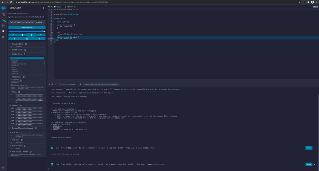
The Remix IDE has a similar capability. Once a transaction has been executed and is displayed on the main screen, you can click on the blue “Debug” icon next to the transaction, and a debugger window will open on the left of the screen. You can now step forward and back, inspect opcodes, stack, memory and storage and even set breakpoints. In the Remix IDE, you can even debug deployment transaction, which is not possible in Brownie.
Function selectors
Having all these tools at our disposal, it is now not terribly difficult to understand the actual runtime bytecode. Here is a list of the opcodes, along with a few comments and tags.
// This is the start of the runtime bytecode
// initialize free memory pointer
PUSH1 0x80
PUSH1 0x40
MSTORE
// Repeat the check for a non-zero value
CALLVALUE
DUP1
ISZERO
PUSH1 0xF
// conditionally jump to target 1
JUMPI
PUSH1 0x0
DUP1
REVERT
// This is jump target 1. We get here only
// if the value is zero
JUMPDEST
POP
PUSH1 0x4
CALLDATASIZE
LT
PUSH1 0x28
JUMPI // conditional jump to jump target 2
// We only get here if we have at least four bytes
// of data
PUSH1 0x0
CALLDATALOAD
PUSH1 0xE0
SHR
DUP1
PUSH4
0xEF5FB05B
EQ
PUSH1 0x2D
JUMPI
// This is jump target 2
JUMPDEST
PUSH1 0x0
DUP1
REVERT
// This is jump target 3, here we enter
// the sayHello function
JUMPDEST
PUSH1 0x33  // offset of jump target 4
PUSH1 0x35  // offset of jump target 5
JUMP
// This is jump target 4
JUMPDEST
STOP
// This is jump target 5
// The code starting here is the actual sayHello function
JUMPDEST
PUSH1 0x40
MLOAD
PUSH32 0x3ACB315082DEA2F72DFEEC435F2B0E4DD95A4FD423E89C8CB51DC75FA38D7961
SWAP1
PUSH1 0x0
SWAP1
LOG1
JUMP
I have stripped off a few opcodes at the end which we will take about a bit later. Let us go through the code line by line and try to understand what it does.
The first three lines are familiar – we again initialize the free memory pointer which Solidity stores at memory address 0x40 to its initial value 0x80. Similary, we have already seen the next lines, starting with CALLVALUE, while analyzing the init bytecode. This code again checks that the value of the transaction is zero and reverts if this is not the case, reflecting the fact that our contract does not have a payable function. If the value is zero, the processing continues at the point in the code that I have called jump target 1.
Here, we first clean up the stack by popping the last value. We then push four onto the stack, followed by the output of CALLDATASIZE, which is the length of the transaction input field. The LT opcode compares these two values and pushes the result of the comparison onto the stack. If the result of the comparison is true, i.e. if we have less than four bytes in the input field, we jump to jump target 2, where we again revert.
To understand why this code makes sense, recall that the first four bytes of the input field are supposed to be the hash of the signature of the function we want to call. If we have less than four bytes, the call is not targeting a function, and as we do not have a fallback function, we revert.
If we have at least four bytes of data, we continue at the next line, where we first push zero onto the stack and then run CALLDATALOAD, which loads the first full 32 byte word of the call data onto the stack (the zero that we have just pushed is the offset). We then execute the set of instructions
PUSH1 0xE0 // 0xE0 is 224
SHR
DUP1
PUSH4 0xEF5FB05B
EQ
This looks a bit mysterious, but is actually not too difficult to understand. After the first push, our stack looks as follows.
| 224 | first 32 bytes of transaction input |
When we then execute SHR, which is a shift operation to the right, we shift the second item on the stack by the number of bits specified by the first item to the right, so we shift the 32 bytes, i.e. 256 bits, by 224 bits to the right. This amounts to moving the first 32 bytes to the rightmost position, so that what we now have on the stack are the first four bytes of the input data, i.e. exactly those four bytes that contain the hash of the function signature. We then push four bytes on the stack, so that our stack is now
| 0xEF5FB05B | first four bytes of the function signature |
and use EQ to compare them, so that stack item at the top of the stack is now
first four bytes of function signature == 0xEF5FB05B
Now open Brownie and run
web3.keccak(text="sayHello()")[:4]
to convince yourself that the four bytes to which we compare are exactly the hash of “sayHello()”. Thus, we execute the conditional jump that comes next only if the first four bytes of the input data indicate that we want to call this method, otherwise we continue and hit upon our return statement.
The code that we have just seen therefore realizes the function selection. If your contract contains more than one function, you will see more than one comparison, and the upshot is that we either jump into the function that corresponds to the signature hash or revert (unless we have a fallback function).
This also tells us that in our case, the execution of sayHello() starts at jump target 3. The code that we see here is also typical. We push two values on the stack – first a return offset and then a jump target. We then jump, execute some code and eventually execute another jump. This second jump will then take its target from the stack, so it returns to the first offset that we have pushed onto the stack. In our case, we jump to target 5, execute the code there, and then jump back to target 4. This approach – pushing return values onto the stack – mimics the way how local functions are executed in other programming languages like C. In our case, jump target 4 is simply executing the STOP opcode which completes the execution without a return value.
Finally, let us take a look at the code at jump target 5, which is therefore the body of sayHello(). Here, we first run MLOAD to get the value of the free memory pointer. We then put a full 32 byte word onto the stack, namely the hash of the string “SayHello()'”, i.e. the signature of the event that we emit. We then swap the first two elements on the stack, push zero and swap once more. Our stack now looks as follows.
| 0x80 | 0x0 | hash(event signature) | return address |
Now we execute LOG1. Again, the yellow paper is our friend and tells us that the first entry on the stack is the offset of the log data, the second entry is the length and the third entry is the first (and, in this case, the only) topic. So we log an event with no data and topic being the hash of the event signature, as expected. The log statement will consume the first three stack items, and when we now jump, we therefore end up at tag 4, where we execute the STOP opcode to complete the transaction.
Encoding and state variables
We have now completed the analysis of our sample contract. A natural next step is to add more functionality to the contract and see how this changes the output of the compile. As an example, let us add some state to our contract. In the body of the contract code, add the line
uint256 value;
and the method
function store(uint256 _value) public {
    value = _value;
}
Let us now run the compiler again, this time with a few more flags that request additional output (the reason for this will become clear in a minute).
$SOLC contracts/Hello.sol \
       --asm \
       --optimize \
       --storage-layout \
       --combined-json generated-sources-runtime
Here is a listing of the relevant code that is newly added to our contract by the changes we have made. Again, I have added some comments and labeled the jump destinations from A to E.
PUSH1 0x47     // address of label B
PUSH1 0x42     // address of label A
CALLDATASIZE
PUSH1 0x4
PUSH1 0x76     // address of label D
JUMP
// Label A - this is at offset 0x42
JUMPDEST
PUSH1 0x0
SSTORE
JUMP
// Label B - this is at offset 0x47
JUMPDEST
STOP
// Label C - this is at offset 0x48
// I have removed the code in this  section
// which we have already looked at before
// it logs the event and then jumps to label B
// where we STOP
// Label D - this is at offset 0x76
JUMPDEST
PUSH1 0x0
PUSH1 0x20
DUP3
DUP5
SUB
SLT
ISZERO
PUSH1 0x87     // address of label E
JUMPI          // conditional jump to label E
PUSH1 0x0
DUP1
REVERT
// Label E - this is at offset 0x87
JUMPDEST
POP
CALLDATALOAD
SWAP2
SWAP1
POP
JUMP
The first few lines are again easy to interpret – we prepare a jump, which is an internal function call, i.e. we place a return address and, in this case, arguments on the stack and then jump to label D. When we get there, our stack looks as follows (recall that CALLDATASIZE puts the size of the calldata, i.e. the length of the transaction input in bytes, onto the stack).
4 | len(tx.input) | label A | label B
At label D, we put a few additional items on the stack. If you go through the instructions, you will find that when we reach the SUB opcode, the stack looks as follows.
len(tx.input) | 4 | 32 | 0 | 4 | len(tx.input) | A | B
Now we execute the SUB opcode, which will pop the first two items off the stack and push their difference. Thus, after completing this opcode, our stack will be
len(tx.input) - 4 | 32 | 0 | 4 | len(tx.input) | A | B
The next instruction, SLT, is a signed version of the less-than instruction that we have already seen. Together with the subsequent ISZERO which is a simple logical inversion, its impact is to provide the following stack.
!(len(tx.input) - 4 < 32) | 0 | 4 | len(tx.input) | A | B
To get an idea what this is supposed to do, looking at the assembler output helps. In the comments that Solidity has generated, we find a hint – utility.yul. As the Solidity documentation explains, this means that the code we are looking at is part of a library of utility functions, written in the Yul language (an intermediate language that Solidity uses internally). However, these utility functions are not stored anywhere in a file with this name, but are actually generated on the fly by the compiler (in our case, this happens here). The additional flag generated-source-runtime that we have used when running Solidity instructs the compiler to print out a Yul representation of the utility functions. The Yul code, the name of the function and the source code of the Solidity compiler that I have linked above solve the puzzle – the code we are looking at is supposed to decode the transaction input and to extract the argument (which is called _value in the source code of our contract).
Now the Solidity ABI demands that the argument be stored in the transaction input as a 256-bit, i.e. 32 byte word, directly after the four bytes containing the function signature. What the code that we are analyzing is doing is to check that the total length of the transaction input is at least those four bytes plus the 32 bytes. If this is not the case, we continue and revert. If this is the case, i.e. if the validation is successful, we perform a conditional jump and end up at label E. When we get there, our stack is
0 | 4 | len(tx.input) | A | B
We now remove the first item on the stack, use CALLDATALOAD to load a full 32 byte word starting at byte 4 of the transaction input onto the stack (i.e. the 32 byte word that is supposed to contain our parameter), and use two swaps and a pop operation to produce the following stack.
A | _value | B
The conditional jump will therefore take us to label A again, with the _value parameter at the top of the stack. Hee, we push zero onto the stack and perform an SSTORE. This will store _value at position zero of the storage and leave us with the address of label B on the stack. The following jump will therefore take us to the STOP opcode, and the transaction completes.
So, the content at offset zero of the storage seems to represent the stored value. Here, we could easily derive this from the code, but in general, this can be more difficult. To help us to map the state variables declared in the source code to storage locations, Solidity creates a storage map which we have included in our output using the –storage-layout switch. The storage layout is an array, where each entry represents one state variable. For each variable, there is a slot and an offset. As indicated in the documentation, the slot is the address in the storage area, but one slot can contain more than one item (if an item is smaller than 32 bytes), and in this case, the offset is the offset within the slot. For dynamic data types, the layout is much more complicated, for mappings, for instance, the actual slot is determined as a hash value of he key.
Metadata and hashes
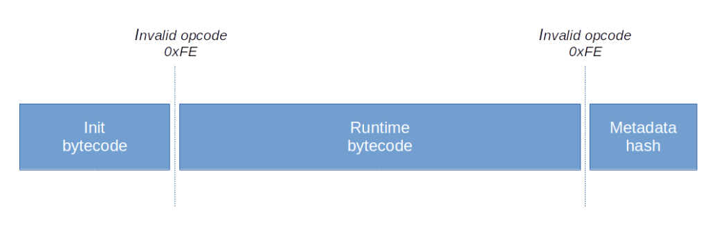
If you have followed the analysis carefully, you might have noted that the last few opcodes do not seem to be executed at all. In fact, they do not even make sense, starting already with an invalid opcode 0xFE. Again, the assembler output helps to interpret this – it designates this part of the bytecode as “auxdata”, which does in fact not contain valid bytecode, but the IFPS hash of the contract metadata (more precisely a CBOR encoded structure which contains the IPFS hash as a key)
The contract metadata, which can be produced using the –metadata compiler switch, is a JSON structure that contains, among other things
- the contract ABI
- the Keccak hash of the source code
- the IPFS hash of the source code
- the exact compiler version
- the compiler settings used to produce the bytecode
The idea behind this is that a developer can store the metadata and the contract source in IPFS. A user who finds the contract on the blockchain can then use the last few bytes – the IPFS hash of the metadata – to retrieve that document from the IPFS network. As the metadata document contains the IPFS hash of the source, a user could now retrieve the source as well. This mechanism therefore allows you to link the source code to the contract and to prove that the contract bytecode has been created using the source code and a given set of compiler settings. Within the Solidity source code, all this happens here.
We have seen that the metadata hash and the runtime bytecode are separated by the invalid opcode 0xFE. This byte appears at another location in the full bytecode – the end of the init bytecode. In both cases, the motivation is the same – we want to avoid that, due to an error, the execution can continue past these boundaries. So we now realize that the full bytecode contains of three sections, separated by the invalid opcode 0xFE.
This closes our post for today. Of course, you could now add additional features to our contract, maybe return values or mappings, and see how this affects the generated bytecode. In the next post, however, we will turn to another topic which is central to understanding smart contracts – how the Ethereum virtual machine actually operates.

2 Comments