
In the last post, we have looked a bit at the theory behind elliptic curves. In this post, we will now see how all this works down to earth and use Python to actually run some calculations.
The first thing that we need is an explicit formula for the addition of two points on an elliptic curve. We will not derive this here, but simply give you the result – see for instance [1] for more details. Given two points 


inv = inv_mod_p(x2 - x1, p)
x3 = ((y2 - y1)*inv)**2 - x1 - x2
y3 = (y2 - y1)*inv*(x1 - x3) - y1
Here we assume that we have a function inv_mod that will give us the inverse modulo some prime number p which is the number of elements of our base field. Typically, this can be done using the so-called extended euclidian algorithm.
However, there are a few special cases we need to consider. This is apparent if we look at this formula in more detail – what happens if the inverse does not exist because the points 

This happens if we want to add two points that have the same x-coordinate. There are two cases we need to consider. First, the y-coordinates could be equal as well. Then we are trying to add a point to itself, and we need to apply the formula provided in [1] for that special case. Or the y-coordinate of the second point is minus the y-coordinate of the first point. Then we try to add a point to its own inverse. The result will be the neutral element of the group which is usually called the point at infinity (there is a reason for this: if we embedd the curve into a projective plane, this point will in fact be the intersection of its completion with the line at infinity in the projective plane…).
To describe points on an elliptic curve, we need both coordinates, the x and the y-coordinate. Thus it makes sense to implement a class for this purpose. Instances of this class need to store the x- and y-coordinates and – for convenience – a boolean that tells us whether a point is the point at infinity. So our full code for this class looks as follows.
class CurvePoint:

    def __init__(self, x, y, infinity = False):
        self.x = x
        self.y = y
        self.infinity = infinity

    def __add__(self, other):
        #
        # Capture trivial cases - one of the points is infinity
        #
        if self.infinity:
            return other
        if other.infinity:
            return self
        #
        # First check whether we are adding or doubling
        #
        x1 = self.x
        x2 = other.x
        y1 = self.y
        y2 = other.y
        infinity = False
        if (x1 - x2) % p == 0:
            #
            # Are we talking about doubling or addition
            # of the inverse?
            #
            if (y1 + y2) % p == 0:
                infinity = True
                x3 = 0
                y3 = 0
            else:
                inv = inv_mod_p(2*y1, p)
                x3 = (inv*(3*x1**2 + a))**2 - 2*x1
                y3 = (inv*(3*x1**2 + a))*(x1 - x3) - y1
        else:
            #
            # Standard case
            #
            inv = inv_mod_p(x2 - x1, p)
            x3 = ((y2 - y1)*inv)**2 - x1 - x2
            y3 = (y2 - y1)*inv*(x1 - x3) - y1

        return CurvePoint(x3 % p, y3 % p, infinity)
As already mentioned, that assumes that you have a function inv_mod_p in your namespace to compute the inverse modulo p. It also assumes that the variables p, a and b that describe the curve parameters are somewhere in your global namespace (of course you could introduce a class to represent a curve that stores all this, but let us keep it quick and dirty at this point).
Now having these routines, we can actually do a few example and verify that the outcome is as expected. We use a few examples with low values of p from [1] .
#
# Define curve parameters
#

p = 29
a = 4
b = 20
#
# and add a few points
#
A = CurvePoint(5,22)
B = CurvePoint(16, 27)
O = CurvePoint(0,0,infinity=True)
C = A + B
assert(C.x == 13)
assert(C.y == 6)
assert(C.infinity == False)
C = A + A
assert(C.x == 14)
assert(C.y == 6)
assert(C.infinity == False)
A = CurvePoint(17,19)
B = CurvePoint(17,10)
C = A + B
assert(C.infinity == True)
A = B + O
assert(A.x == B.x)
assert(A.y == B.y)
assert(A.infinity == B.infinity)
A = O + B
assert(A.x == B.x)
assert(A.y == B.y)
assert(A.infinity == B.infinity)
For the sake of demonstration, we have shown how to build elliptic curve arithmetic from scratch. We could now proceed to implement multiplication and the ECDS algorithm ourselves, but as so often, there is a Python library that will do this for us. Well, there is probably more than one, but I like the Python ECDSA library maintained by Brian Warner.
The most basic classes in this library are – you might have guessed that- curves and points. Curves are initialized providing the basic parameters p, a and b. Then points are created by specifying a curve and the x and y coordinates of the points. Thanks to operator overloading, points can then be added and multiplied with integers using standard syntax. Here is a code snippet that reproduces the first of our examples from above using the ECDSA library.
import ecdsa

#
# Create a curve with parameters p,a and b
# with the ECDSA library
#
curve = ecdsa.ellipticcurve.CurveFp(p,a,b)
#
# Define two points and add them
#
A = ecdsa.ellipticcurve.Point(curve, 5, 22)
B = ecdsa.ellipticcurve.Point(curve, 16, 27)
C = A + B
assert(C.x() == 13)
assert(C.y() == 6)
assert(C != ecdsa.ellipticcurve.INFINITY)
Very easy – and very useful. And of course reassuring to see that we get the same result than our hand-crafted code for the arithmetic above gave us.
But this is not yet all, the library can of course do much more. Let us use it to create a signature. For that purpose, we obviously need a reasonable large value for the prime p, otherwise we could easily use a brute-force attack to determine our private key from the public key. In my previous post on the theoretical foundations, I have already mentioned the papers published by the SECG, the Standards for efficient cryptography group. This group has published some standard curves that we can use. One of them is the curve SECP256K1 which is a curve over a prime field 

This curve is the curve which is used by the bitcoin protocol. As many other standardized curves, it is hard-coded in the ECDSA library. To get it, use the following code.
#
# Get the standard curve SECP256K1
# and its parameters
#
curve = ecdsa.curves.SECP256k1
G = curve.generator
p = curve.curve.p()
a = curve.curve.a()
b = curve.curve.b()
n = G.order()
Let us now apply what we have learned about signatures. First, we need a private key and a public key determined from it. Thus we pick a random number that will be our secret and multiply the generator of the curve by it to get our public key.
#
# Determine a private key and a public key
#
d = ecdsa.util.randrange(n-1)
Q = d*G
pKey = ecdsa.ecdsa.Public_key(G, Q)
sKey = ecdsa.ecdsa.Private_key(pKey, d)
Next we need a hash value that we will sign. Usually, we would derive this value from a message using some cryptographic hash function like SHA256, but we will simply simulate this by drawing a random number h. We can then use the method sign of the ECDSA private key object to create a signature. This will return a signature object from which we can retrieve the values r and s.
h = ecdsa.util.randrange(n-1)
k = ecdsa.util.randrange(n-1)
signature = sKey.sign(h, k)
r = signature.r
s = signature.s
Let us verify that the algorithm really works as described the previous post. So we first need to multiply our randomly chosen integer k with the generator of the curve, the number r should then be the x-coordinate of this point. We then invert k modulo n and multiply the result by h + dr. This should give us s.
_r = (k*G).x() % n
assert(_r == r)

w = inv_mod_p(k, n)
_s = ((h+d*r)*w) % n
assert(_s == s)
If you run this code, you will hopefully see that the assertions pass. Our code works, and produces the same result as the ECDSA library. That is already reassuring. Having gone so far, we can now of course also verify the signature – again we do this once using the ECDSA library and once using our own code.
#
# Now we manually verify the signature
#
w = inv_mod_p(s, n)
assert(1 == (w*s % n))
u1 = w * h % n
u2 = w * r % n
X = u1*G + u2*Q
assert(X.x() == r)

#
# Finally we verify the signature using the
# lib
#
assert(pKey.verifies(h, signature) == True)
That is it for today. We have seen how elliptic curves can be used in practice to create and verify digital signatures and have looked at the ECDSA library that offers ready made functions for that purpose. The full source code can by downloaded from GitHub.
In my next post, I will look at the way how private and public ECDSA keys appear in the bitcoin protocol. If you want to learn more and play around a bit with elliptic curves in the meantime, I recommend the online tool [2]. You might also want to take a look at Andrea Corbellinis excellent post on elliptic curve cryptography.
1. D. Hankerson, A. Menezes, S. Vanstone,
Guide to elliptic curve cryptography, Springer, New York 2004
2. Elliptic curve point addition online tool at https://cdn.rawgit.com/andreacorbellini/ecc/920b29a/interactive/modk-add.html
 and encrypt it, i.e. apply a function
  that depends on the key
  to obtain an encrypted message
  .
. to the received message to decrypt it again. If
  and
and  are chosen properly, then they will be inverses of each other, i.e.
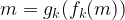
 and
and  to obtain their product
  , it requires a lot of computing power to execute the reverse operation, i.e. to determine
  . The well known RSA algorithm is based on this.
 as well as an integer
  which is obtained by adding performing k additions.
 (most of the time,
  that obeys an equation of the form
 .
.
 and
and  and features a prominent role in the bitcoin protocol (this curve over a certain finite field is known as SECP256K1, more on this in a later post). The blue line visualizes all pairs
  . She then sends that signature along with the original message and her public key to Bob. Using that information, Bob can verify the signature to confirm that it has been created using the private key that belongs to the public key and that the message that he has received is identical to the message that Alice has signed. Assuming that only Alice has access to the private key, he can then deduce that Alice has actually composed and approved the message. In practice, it is not the actual message that is signed, but a hash value of the message to keep the signature short.
 and
and  and some point
  on the curve called the generator. In
  between zero and the order

 . Next Alice picks a random number
  . Let
. Let  denote the x-coordinate of this point. Then Alice determines
 .
. and determine the point


 is equal to the x-coordinate of
  and therefore the secret
